Scaling Width: µP and Hyperparameter Transfer - Coming Soon
Scaling Width: Where the Story Bends - Coming Soon
Why Width
Width
is the number of neurons in a hidden layer, i.e.
hidden_size
in modern LLMs. It is the axis that has grown most during the deep learning (DL) era.
An effect you can ignore at 512 can decide the run at 7168.
So the question is
what changes as width grows.
Does a network of width 7168 train like one of width 512?
Do the initialization and learning rate tuned on the narrow one still work on the wide one?
Mathematics has a standard move for a question like this:
push the parameter to its extreme.
The limit often shows a structure that every finite case hides.
Here that means letting the width go to infinity.
I came to DL from mathematics, and the neural tangent kernel was my way in. This post is based on a talk I gave at a
Deepest
seminar.
Takeaway
At large width, sums over neurons become averages, and the central limit theorem and the law of large numbers take over. Two narrower questions then get clean answers, at a cost.
What is the network at initialization?
As the width grows, a random network's output behaves more and more like a Gaussian process (GP)
[2,3,4].
Its kernel, the NNGP kernel, depends only on the architecture.
What does gradient descent do to it?
Gradient descent on the weights is kernel gradient descent on the function, with a second kernel, the neural tangent kernel (NTK).
As the width grows, the NTK approaches a fixed kernel set by the architecture and changes less and less during training, so training approaches a kernel method
[1].
The cost.
At large width, the NTK barely moves because each weight barely moves.
So wide networks in this regime learn almost no features.
The rest of the series looks for a limit where features keep moving, which leads to µP.
Notation.
The series uses one network throughout: an MLP with input
\xi\in\mathbb{R}^d, hidden width
n, and
L
hidden layers, as in Yang and Hu
[6].
h^l
is the preactivation,
x^l
the activation,
\phi
the nonlinearity.
A subscript on
x^l,
h^l
or
W
picks a neuron: e.g.
x^l_i
is the
i
-th coordinate of
x^l.
W^l
has shape fan-out
\times
fan-in.
There are no biases.
The output is a scalar, so
W^{L+1}\in\mathbb{R}^{1\times n}.
\theta\in\mathbb{R}^P
stacks every entry of every
W^l.
\mathcal{L}
is the loss and
\eta
the learning rate.
The training set is
\xi_1,\ldots,\xi_N
with labels
y_1,\ldots,y_N.
\mathcal{X}
and
\mathcal{Y}
stack them, and
f(\mathcal{X})\in\mathbb{R}^N
stacks the
f(\xi_j).
K_t
is the NTK at training time
t, and
K_\infty
its infinite-width limit.
\Sigma
is the NNGP kernel.
\Theta(\cdot)means asymptotic order
and nothing else.
Many papers, Jacot et al. among them, use
Θ
for the NTK. I convert their notation to
K.
Every kernel in the post (
K_t,
K_\infty,
\Sigma,
\dot\Sigma
and their layer-wise versions) is a map
\mathbb{R}^d\times\mathbb{R}^d\to\mathbb{R}.
Its arguments are written
\xi,\xi', because
x
is taken by the activations. They stand for any input, test inputs included.
A subscript on
\xi
picks a training point:
\xi_j
is the
j
-th of
\xi_1,\ldots,\xi_N.
A prime on
\xi
only marks a second input. A prime on
\phi
is its derivative.
Given sets of inputs, a kernel returns a matrix:
K(\mathcal{A},\mathcal{B})
has entries
K(a,b), so
K(\mathcal{X},\mathcal{X})\in\mathbb{R}^{N\times N}
and
K(\xi,\mathcal{X})\in\mathbb{R}^{1\times N}.
Where the 1/√n Sits
Every hidden layer has width
n, and
n\to\infty
grows them all together. Even so, "let
n\to\infty
" means nothing until you say what else scales with
n.
A
parametrization
fixes three things per layer: where a width factor multiplies the weight, the variance at initialization, and the learning rate. Two parametrizations matter in this post.
Standard parametrization (SP).
This is the PyTorch default. The trainable matrix is the weight itself, initialized with variance 1/fan-in:
Lower-case
w
is the trainable parameter, and
W=w/\sqrt{n}
is the effective weight.
Jacot et al. and Lee et al. use this form, with biases added
[1,5]. This post drops the biases.
The first layer divides by
\sqrt{d}.
At initialization the two are the same network:
w/\sqrt{n}
has variance
1/n, exactly like SP's
W.
Lee et al. say it directly: "the function that the network represents is the same for both NTK and standard parameterization, training dynamics under gradient descent are generally different"
[5].
They part under gradient descent, because gradient descent updates the trainable matrix, and that matrix differs. Take a layer with fan-in
n.
In NTP,
W=w/\sqrt{n}, so one step picks up the factor
1/\sqrt{n}
twice:
The step is
\Delta w=-\eta\,\partial\mathcal{L}/\partial w, and by the chain rule
\partial\mathcal{L}/\partial w=\dfrac{1}{\sqrt{n}}\,\partial\mathcal{L}/\partial W.
That step moves
W
by only
\Delta W=\Delta w/\sqrt{n}.
One step of size
\eta
therefore moves the effective weight by
This is the whole network, not only its last layer: every layer below sits inside
x^L_i(\xi). Writing out the last sum is what makes the limit visible.
Why it becomes Gaussian:
Fix the lower layers, so
x^L(\xi)
is a fixed vector. Write
W_i=W^{L+1}_{1i}.
The
W_i
are drawn independently of the lower layers, and of each other, with mean
0
and variance
1/n.
So
f_0(\xi)=\sum_i W_i\,x^L_i(\xi)
is a sum of independent Gaussians times fixed numbers. It is exactly Gaussian, with mean
0.
Its covariance keeps only the
i=j
terms, because
\mathbb{E}[W_iW_j]=0
for
i\neq j
and
\mathbb{E}[W_i^2]=1/n:
Run the same argument up from the input, one layer at a time. For Lipschitz
\phi, each such average converges to a deterministic limit as the widths grow one layer after another
[1].
Matthews et al. prove the same GP limit, for a broad class of
\phi, with all widths growing together
[4].
So, as the widths grow,
f_0
at any finite set of inputs tends in law to a Gaussian vector whose covariance does not depend on the weights drawn.
A random function whose values at every finite set of inputs are jointly Gaussian is a GP.
From here on, the post leans on GP facts at almost every step. If you are not familiar with them, read
About Gaussian Process
first. It covers the four this post uses most:
A kernel is the covariance of a GP, and it must be positive semi-definite. Both the NNGP kernel and the NTK are kernels in this sense.
Conditioning a GP on data
gives the posterior mean. The NNGP's Bayesian posterior below is exactly this.
Kernel ridge regression and its ridgeless limit.
As the width grows, the law of a trained network's prediction tends to a Gaussian whose mean is this.
The weight-space view, where a kernel is an inner product of features. The NTK is read this way, with the parameter gradient as the feature map.
Neal proved this GP limit for one hidden layer
[2]. Lee et al. and Matthews et al. extended it to deep networks
[3,4]. Jacot et al. turn the layer-by-layer argument into a recursion
[1]:
At finite width,
h^l_i(\xi)
depends on
\xi
through
l
random weight matrices and
l-1
applications of
\phi.
Given the layer below, the coordinates
h^l_1,\ldots,h^l_n
are i.i.d. and Gaussian across inputs, as for
f_0. Their covariance is an average over the layer below, so it converges to a deterministic
\Sigma^{(l)}.
So
\dfrac{1}{n}\sum_i\phi(h^l_i(\xi))\,\phi(h^l_i(\xi'))
averages
n
independent copies and converges to
\mathbb{E}[\phi(g(\xi))\,\phi(g(\xi'))].
Here
g, the limit in law of each
h^l_i, is a zero-mean GP with covariance
\Sigma^{(l)}.
That expectation is the covariance of
h^{l+1}.
💡
As the width grows, eachh^l_itends in law to a GP whose law depends on\xionly through\Sigma^{(l)}. Everything the firstllayers did to\xiis summarized by that kernel, so the next layer needs nothing else.
The first layer has no nonlinearity below it, so
\Sigma^{(1)}
is the linear kernel scaled by
1/d, the first layer's fan-in. The output is layer
L+1, so the
NNGP kernel
is
\Sigma=\Sigma^{(L+1)}: the covariance of the GP that
f_0
tends to in law as the widths grow.
Two things make this useful.
Bayesian inference becomes exact.
Condition the Gaussian process on
f(\mathcal{X})=\mathcal{Y}. If
\Sigma(\mathcal{X},\mathcal{X})
is invertible, the posterior mean is
\Sigma(\xi,\mathcal{X})\,\Sigma(\mathcal{X},\mathcal{X})^{-1}\mathcal{Y}
[5].
The kernel depends only on the architecture.
\phi
and depth fix
\Sigma. No sample of weights enters it.
💡
The NNGP kernelΣis the covariance of the GP that a randomly initialized network's output tends to as the width grows. The architecture alone sets it.
The Network Under Gradient Descent: NTK
The NTK answers the Takeaway's second question, what gradient descent does to the network. The route there is a change of viewpoint:
stop tracking\thetaand trackf_\thetainstead.
Gradient flow.
Gradient descent is
\theta_{k+1}=\theta_k-\eta\nabla_\theta\mathcal{L}(\theta_k). Read it as one Euler step of an ordinary differential equation. Shrinking the step gives
gradient flow:
The loss over the training set is
\mathcal{L}(\theta)=\dfrac{1}{N}\sum_{j}\ell(f_\theta(\xi_j),y_j).
It sees
\theta
only through
f_\theta, so
\mathcal{L}
can be read as a functional on a space of functions.
Its gradient with respect to
f
at a training point is
\nabla_f\ell(\xi_j)=\partial\ell/\partial f, evaluated at
(f_\theta(\xi_j),y_j). For squared error, it is the residual
f_\theta(\xi_j)-y_j.
Kernel gradient flow.
Write the
Jacobian
of the output at input
\xi
as
This is the
neural tangent kernel
[1]. It is Lee et al.'s Eq. (4) and Jacot et al.'s definition,
specialized to scalar output.
⚠️
Assumption: gradient flow updates every parameter.
Papers disagree on what "the NTK" names: the function
K_t, its
N\times N
Gram matrix on the training set, or the infinite-width limit. This post fixes the names:
The NTK
is the function
K_t, at any width and time.
This is
kernel gradient descent: the functional gradient on the data, smoothed by a kernel. It has the same form as Jacot et al.'s kernel gradient
[1], with
\eta
written out.
💡
Gradient descent on the parameters is kernel gradient descent on the function, with kernelK_t = J Jᵀ.
Four readings of this equation carry the rest of the post.
Parameters left the right-hand side.
They survive only inside
K_t.
Gradient descent now reads as an equation forf, withK_tas its only link to\theta.
The kernel gradient is defined everywhere.
The ordinary gradient lives on the
N
training points. The kernel gradient is defined at any
\xi, including test inputs. That is how fitting
\mathcal{X}
moves predictions off
\mathcal{X}.
The feature map is the parameter gradient.
In kernel-method terms,
K_t(\xi,\xi')=\langle\varphi(\xi),\varphi(\xi')\rangle
with feature map
\varphi(\cdot)=\nabla_\theta f_{\theta(t)}(\cdot)\in\mathbb{R}^P.
K_tdepends on\theta(t).
At finite width it moves as the parameters move, so the equation is not closed. It is exact, and so far it is useless.
Why SP needs a learning rate∝ 1/n
The NTK is a sum over parameters. Call
K^{\text{out}}
the part of that sum over the
n
output weights.
Under NTP:
f=n^{-1/2}\sum_i w^{L+1}_i x^L_i, so
\partial f(\xi)/\partial w^{L+1}_i=x^L_i(\xi)/\sqrt{n}.
K^{\text{out}}(\xi,\xi')=\dfrac{1}{n}\sum_{i=1}^{n}x^L_i(\xi)\,x^L_i(\xi'), an average of
n
terms.
It converges to
\Sigma^{(L+1)}(\xi,\xi'), which is
\Theta(1).
Under SP:
f=\sum_i W^{L+1}_{1i}x^L_i, so
\partial f(\xi)/\partial W^{L+1}_{1i}=x^L_i(\xi).
K^{\text{out}}(\xi,\xi')=\sum_{i=1}^{n}x^L_i(\xi)\,x^L_i(\xi'), a sum rather than an average.
It grows like
n\,\Sigma^{(L+1)}(\xi,\xi').
The kernel sets how fast
f
moves per unit of
\eta.
An SP kernel that grows like
n
needs
\eta\propto1/n
to keep the function's motion finite.
That
1/n
is exactly the factor NTP builds into its forward pass.
As Width Grows, the Kernel Barely Moves
Two theorems by Jacot et al. close the equation
[1]. Both are stated for NTP, with the widths growing one layer after another. Lee et al. obtain both results again with all widths equal to
n
and growing together
[5].
Theorem 1: the kernel at initialization tends to a deterministic one.
Take a Lipschitz
\phi
and let the hidden widths go to infinity one layer after another, as Jacot et al. do. The NTK at initialization converges in probability to a deterministic kernel
K_\infty
[1]. Here
K^{(l)}_\infty
is the limiting NTK of one neuron
h^l_i, the same for every
i, and
\dot\Sigma
is built like
\Sigma, with the derivative
\phi'
in place of
\phi:
The network's limiting NTK is
K_\infty=K^{(L+1)}_\infty. The product is pointwise in
(\xi,\xi').
It depends on the architecture only.
The random draw of weights has averaged out.
It contains the NNGP kernel.
At
l=L, the recursion reads
K_\infty=\Sigma+K^{(L)}_\infty\,\dot\Sigma^{(L+1)}.
Theorem 2: as the width grows, the kernel moves less and less during training.
Let
\phi
also be twice differentiable with bounded second derivative. Train every parameter by gradient flow up to any fixed time
T, as long as the total size of the loss gradient,
\int_0^T\|\nabla_f\ell\|\,dt, stays bounded in probability as the widths grow.
Then, as the widths go to infinity one layer after another,
K_t\to K_\infty
in probability, uniformly for
t\in[0,T]
[1].
The limit is in width, not in time.
Training does not drive
K_t
toward
K_\infty.
At every
t
up to
T, a wide enough network's kernel is close to
K_\infty
with high probability, so it barely moves during training.
So as the width grows,
f_t
converges to
\bar f_t, the solution of the same equation with
K_\infty
in place of
K_t:
This is a linear ODE in
\bar f
for squared error. What the fixed kernel changes is easy to miss:
For a convex
\ell, the loss is convex in
f
at every width. It is non-convex in
\theta
only because
f_\theta
depends on
\theta
nonlinearly.
At finite width,
f
moves with
K_t, which depends on
\theta(t). The non-convexity in
\theta
reaches
f
's motion through that kernel.
As width grows,
f_t
converges to the kernel-gradient-descent trajectory with the fixed
K_\infty, on a loss convex in
f. The shape of the loss in
\theta
drops out of the limit.
The effect does not depend on NTP. Lee et al. show the kernel also barely moves under SP with learning rate
\eta/n
[5].
💡
As width grows, the NTK moves less and less during training, and it approaches a kernel set by the architecture alone.
A Wide Network Stays Close to Its Linearization
A constant kernel has a second reading. Which model's tangent kernel stays
K_0
throughout training? The simplest one, the network's first-order expansion around initialization, keeps its parameter gradient fixed at
\nabla_\theta f_0
[5]:
If the kernel does not move,
K_t=K_0
and the two equations coincide, so they trace the same function.
As width grows,
K_t
and
K_0
both approach
K_\infty
for every
t\in[0,T], so the gap between
f_t
and
f^{\mathrm{lin}}_t
goes to zero. This is the limiting NTK seen from parameter space.
The payoff:
f^{\mathrm{lin}}
is linear in
\theta, on the fixed features
\nabla_\theta f_0, so under squared error its training has a closed form, derived below.
What "infinite width" means here.
No network with infinitely many parameters is ever trained.
Every network has a finite width
n
and finitely many parameters. "At infinite width" describes what happens as
n\to\infty.
K(\mathcal{X},\mathcal{X})
is an
N\times N
matrix and
f(\mathcal{X})
an
N
-vector at every width, so they can converge.
\theta
gets longer as
n
grows, so it cannot. That is why this post follows
f
and
K, not
\theta.
How close at finite width.
So far the gap vanishes only in the limit. Lee et al. bound how far a width-
n
network is from it
[5].
Assume squared error, equal hidden widths,
\phi'
bounded and Lipschitz, distinct training inputs, a positive-definite
K_\infty(\mathcal{X},\mathcal{X}), a learning rate below
2/(\lambda_{\min}+\lambda_{\max}), where
\lambda_{\min},\lambda_{\max}
are the extreme eigenvalues of
K_\infty(\mathcal{X},\mathcal{X}), and a test input with
\|\xi\|\le1.
Then three quantities are all
O(n^{-1/2})
with high probability:
The gap
\sup_t|f_t(\xi)-f^{\mathrm{lin}}_t(\xi)|.
The kernel drift
\sup_t\|K_t-K_0\|_F
on the training set.
The weight displacement
\sup_t\|\theta_t-\theta_0\|_2/\sqrt{n}.
Practical reading.
Under NTP, the wider the network, the less its weights and kernel move, so training stays closer to a kernel method on the fixed features
\nabla_\theta f_0.
The loss still falls.
Lowering it needs
f
to move
O(1), not each weight, and many tiny weight changes add up to that.
Closed-Form Dynamics Under Squared Error
Take
\ell(\hat y,y)=\dfrac{1}{2}\|\hat y-y\|_2^2
and write
K_0
for the Gram matrix
K_0(\mathcal{X},\mathcal{X}). Likewise
K_\infty
in
K_\infty^{-1}
and
e^{-\eta K_\infty t}
means
K_\infty(\mathcal{X},\mathcal{X}). The kernel equation becomes a linear ODE with constant coefficients, so it solves in closed form
[5]. On the training points:
If
K_0
is positive definite,
e^{-\eta K_0 t}
decays to
0
as training runs, so
f^{\mathrm{lin}}_t
converges. A subscript
\star
marks the converged value:
It is
\hat f(\xi)=\sum_i(K_0^{-1}\mathcal{Y})_i\,K_0(\xi_i,\xi), ridgeless kernel regression with kernel
K_0.
As
n\to\infty, the law of a trained width-
n
network's prediction tends to a Gaussian whose mean is kernel regression with
K_\infty.
\gamma_\staris what initialization leaves behind.
On the training set,
\gamma_\star(\mathcal{X})=f_0(\mathcal{X})-K_0K_0^{-1}f_0(\mathcal{X})=0. At a test input it is in general nonzero.
f^{\mathrm{lin}}_\star=\mu_\star+\gamma_\star
is spread symmetrically around
\mu_\star: flipping the signs of the output weights keeps the law of
\theta, leaves
K_0
and
\mu_\star
unchanged, and negates
\gamma_\star.
As
n\to\infty,
K_0
tends to
K_\infty, and at each
t
the law of
f^{\mathrm{lin}}_t(\mathcal{X}_{\mathrm{test}})
over initializations tends to a Gaussian with mean
[5]:
K_\infty
is computed through Gaussian expectations. It has closed forms for ReLU and erf
[5], and the Neural Tangents library computes it for common architectures
[7].
Python Implementation and Result
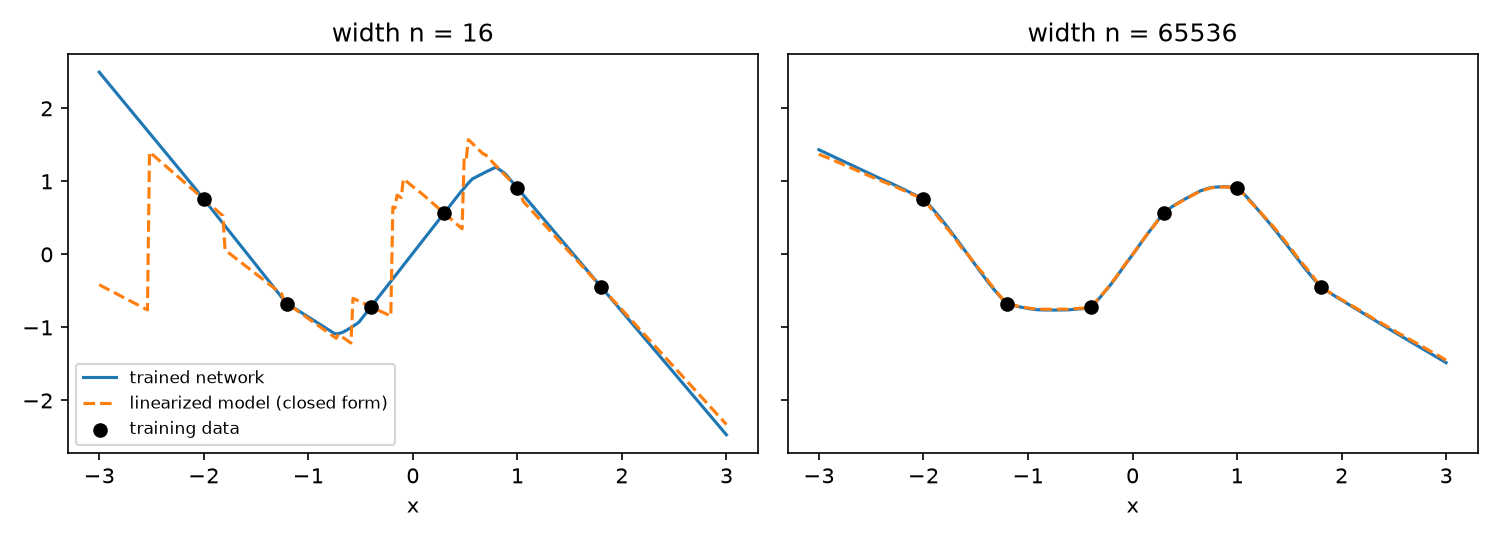
The code below trains a one-hidden-layer ReLU network under NTP on six points of
\sin(2x), at widths 16 and 65536, and compares it with the closed-form linearized model. ReLU is not differentiable at 0, so Theorem 2 and Lee et al.'s bound do not cover it. The plot is an empirical check.
Input.\xi=(x,1), so
d=2.
The network has no biases, so this is the usual bias trick: the weight on the constant coordinate acts as a first-layer bias,
w\cdot(x,1)=w_1x+w_2.
Discrete steps.
Gradient descent replaces
e^{-\eta K_0 t}
with
(I-\eta K_0)^k
after
k
steps
[5].
Code Snippet
import matplotlib.pyplot as plt
import numpy as np

rng = np.random.default_rng(0)


def relu(z):
    return np.maximum(z, 0.0)


def step(z):
    return (z > 0).astype(float)  # derivative of relu


def features(x):
    # xi = (x, 1): the constant coordinate lets the first layer shift its kinks
    return np.stack([x, np.ones_like(x)], axis=1)


def forward(w, v, xi):
    # NTP with one hidden layer: h = w xi / sqrt(d), f = v . relu(h) / sqrt(n)
    h = xi @ w.T / np.sqrt(xi.shape[1])
    return relu(h) @ v / np.sqrt(len(v)), h


def ntk(w, v, xi_a, xi_b):
    # K(xi, xi') = <grad_theta f(xi), grad_theta f(xi')>, summed over v and w
    n, d = w.shape
    _, h_a = forward(w, v, xi_a)
    _, h_b = forward(w, v, xi_b)
    k_v = relu(h_a) @ relu(h_b).T / n
    k_w = (step(h_a) * v**2) @ step(h_b).T / n * (xi_a @ xi_b.T) / d
    return k_v + k_w


x_train = np.array([-2.0, -1.2, -0.4, 0.3, 1.0, 1.8])
y_train = np.sin(2 * x_train)
x_test = np.linspace(-3, 3, 300)
xi_train, xi_test = features(x_train), features(x_test)
eta, T = 0.25, 4000

fig, axes = plt.subplots(1, 2, figsize=(10, 3.6), sharey=True)
for ax, n in zip(axes, [16, 65536]):
    w = rng.standard_normal((n, 2))
    v = rng.standard_normal(n)
    f0_train, _ = forward(w, v, xi_train)
    f0_test, _ = forward(w, v, xi_test)

    # Linearized model after T steps of gradient descent on 1/2 ||f - y||^2:
    # f_lin = f0 + K0(xi, X) K0^{-1} (I - (I - eta K0)^T) (Y - f0(X))
    K0 = ntk(w, v, xi_train, xi_train)
    decay = np.linalg.matrix_power(np.eye(len(x_train)) - eta * K0, T)
    shrink = np.linalg.solve(K0, (np.eye(len(x_train)) - decay) @ (y_train - f0_train))
    f_lin = f0_test + ntk(w, v, xi_test, xi_train) @ shrink

    # The real network, trained by the same T steps of gradient descent
    for _ in range(T):
        f, h = forward(w, v, xi_train)
        r = f - y_train  # dL/df for each training point
        grad_v = relu(h).T @ r / np.sqrt(n)
        grad_w = (
            ((r[:, None] * step(h) * v) / np.sqrt(n)).T
            @ xi_train
            / np.sqrt(xi_train.shape[1])
        )
        v -= eta * grad_v
        w -= eta * grad_w
    f_net, _ = forward(w, v, xi_test)

    ax.plot(x_test, f_net, label="trained network")
    ax.plot(x_test, f_lin, "--", label="linearized model (closed form)")
    ax.scatter(x_train, y_train, color="k", zorder=3, label="training data")
    ax.set_title(f"width n = {n}")
    ax.set_xlabel("x")

axes[0].legend(loc="lower left", fontsize=8)
fig.tight_layout()
fig.savefig("ntk_linearization.png", dpi=150)
Result
At width 16 the two disagree. The linearized model jumps at each neuron's ReLU kink, because its feature map
\nabla_\theta f_0
contains the ReLU's step.
At width 65536 each jump is typically
O(1/n), too small to see.
The real network's kernel also barely moves, so the two curves nearly coincide.
Two Kernels, Two Gaussian Processes
Both kernels are now on the table, and they are easy to blur.
NNGP\Sigma
is the infinite-width covariance of
f_0
over random initializations. It needs only the forward pass.
NTKK_t
is the inner product of one network's parameter gradients, at any width and time.
K_\infty
is its infinite-width limit.
Each route gives a GP for the prediction after seeing the data.
One comes from conditioning the NNGP prior.
The other comes from training one network at each width
n
and letting
n
grow.
Both are compared through
About Gaussian Process
: conditioning a prior
\mathcal{GP}(m,k)
on
f(\mathcal{X})=\mathcal{Y}, with
k(\mathcal{X},\mathcal{X})
invertible, gives the posterior
\mathcal{GP}(m_{\mathcal{D}},k_{\mathcal{D}})
with
The trained network.
For each width
n, initialize a fresh network at random and train it until training converges, under the conditions of "How close at finite width". Its prediction is random, through the initialization.
As
n\to\infty, the law of that prediction tends to a GP
[5]. Its mean is
\mu_\star
from the closed-form section, with
K_0
replaced by
K_\infty:
Its covariance comes from
\gamma_\star, which combines
f_0
(law tending to
\mathcal{GP}(0,\Sigma)
) with
K_0
(tending to
K_\infty
). So it mixes the two kernels and in general is not
k_{\mathcal{D}}
with
k=\Sigma
or
k=K_\infty
[5].
The two means use the same formula. Only the kernel differs:
\Sigma
in one,
K_\infty
in the other.
HowK_\inftydiffers from\Sigma.
At width
n, split the NTK's sum over parameters into the output weights and all the others. Under NTP,
\partial f(\xi)/\partial w^{L+1}_i=x^L_i(\xi)/\sqrt{n}, so
K_0(\xi,\xi')=\underbrace{\dfrac{1}{n}\sum_{i=1}^{n}x^L_i(\xi)\,x^L_i(\xi')}_{\text{output weights}}+\underbrace{\sum_{p\,\notin\,\text{output}}\dfrac{\partial f(\xi)}{\partial\theta_p}\,\dfrac{\partial f(\xi')}{\partial\theta_p}}_{\text{all other weights}}
As
n\to\infty, the first term tends to
\Sigma
and the second to
K^{(L)}_\infty\dot\Sigma^{(L+1)}
(Theorem 1):
The limit of the second term,
K^{(L)}_\infty\dot\Sigma^{(L+1)}, is the whole difference.
Removing the second term from training.
This drops the ⚠️ assumption under the NTK definition.
So far every parameter was trained, so the kernel that drives training was the full NTK.
For each width
n, initialize a fresh network at random and
freeze every weight except the output weights.
Frozen weights have
\dot\theta_p=0
and drop out of the chain rule
df_t(\xi)/dt=\sum_p\partial f_t(\xi)/\partial\theta_p\,\dot\theta_p.
The kernel that drives training is then only the first term,
\dfrac{1}{n}\sum_i x^L_i(\xi)\,x^L_i(\xi'). It never changes, because
x^L
never moves.
As
n\to\infty, that kernel tends to
\Sigma, and the law of the converged prediction tends to the NNGP posterior
\mathcal{GP}(m_{\mathcal{D}},k_{\mathcal{D}})
[4,5].
So in the limit,
\Sigma
is the kernel that drives training when only the output weights train, which nobody does in practice, and
K_\infty
when every weight trains.
💡
The NNGP posterior and the trained network's limiting prediction are both GPs whose mean is kernel regression, with\Sigmain one andK_\inftyin the other. Their covariances differ.
What the Kernel Regime Explains and Costs
What It Explains
Global convergence.
The loss is non-convex in
\theta, yet a wide network still fits the training data. Three steps show why. Start from the linearized model's residual on the training points:
It shrinks at least as fast as
e^{-\eta\lambda t}, with
\lambda
the smallest eigenvalue of
K_0.
Under the conditions of "How close at finite width", Lee et al. show the wide network's own residual also decays exponentially
[5], so its training loss goes to zero.
K_0is positive definite at large width ifK_\inftyis.
K_0\to K_\infty
in probability, so this holds with high probability.
K_\inftyis positive definite for networks with biases.
Jacot et al. prove it for distinct inputs on the unit sphere and any non-polynomial Lipschitz
\phi
[1].
Without biases it can fail. An odd
\phi
such as tanh gives
f(-\xi)=-f(\xi), so targets with
y(-\xi)\neq-y(\xi)
are unreachable, and the kernel is singular on that pair. This post's bias-free network has no such guarantee.
💡
As the width grows, non-convexity inθstops mattering. Training approaches linear regression on fixed features, which fits the data whenever the kernel is positive definite.
What It Costs
What makes the analysis work also breaks it as a model of deep learning.
Each weight barely moves, yet the function does.
Take the NTP output layer.
Each weight starts at size
O(1). Its gradient is
\partial f/\partial w^{L+1}_i=x^L_i/\sqrt{n}, so it moves by
O(n^{-1/2})
over a training run of fixed length.
Lee et al. measure it: the relative change in input and output weights scales as
1/\sqrt{n}, and in intermediate weights as
1/n
[5].
The function still moves by
O(1):
\Delta f=n^{-1/2}\sum_i\Delta w^{L+1}_i\,x^L_i
adds
n
terms of size
O(n^{-1/2})
and divides by
\sqrt{n}.
Each feature coordinate barely moves either.
The last hidden activation
x^L(\xi)
is the network's representation of
\xi.
Yang and Hu argue each of its coordinates changes by
\Theta(n^{-1/2})
in NTP, for a smooth
\phi
such as tanh and a fixed number of SGD steps
[6].
Jacot et al. say the same of activations: "the variation during training of the individual activations in the hidden layers shrinks as their width grows. However their collective variation is significant"
[1].
Yang and Hu name the consequence.
In the NTK limit, "(last layer) features learned during pretraining are essentially the same as those from random initialization"
[6].
Their Word2Vec experiment shows NTK embeddings that are "essentially random"
[6].
Pretraining, transfer and fine-tuning all rest on learned features, so they call this "a fatal weakness of the NTK theory as a model of neural networks in practice"
[6].
Chizat et al. call this regime
lazy training
[8].
About Muon: Why Not Adam?
met the same effect from the optimizer side: a model trained under standard parametrization barely leaves where it started.
Python Implementation and Result
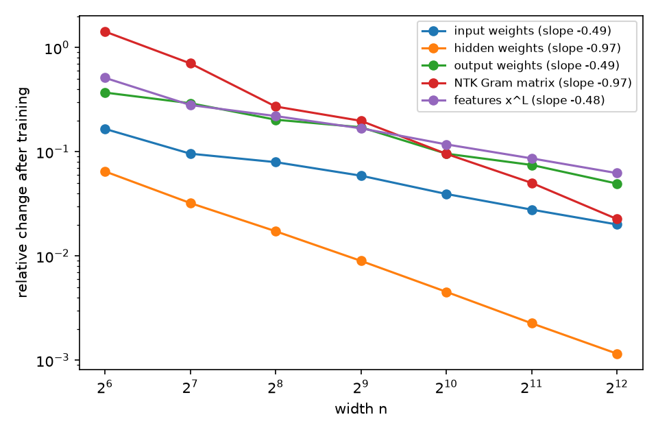
The following code trains a 3-hidden-layer ReLU network under NTP at widths
2^6
to
2^{12}, with the same
\eta
and number of steps, on 128 random inputs.
It then measures how far each part moved, relative to where it started, and fits the exponent of
n.
Code Snippet
import matplotlib.pyplot as plt
import numpy as np
import torch

torch.manual_seed(0)
N, d, L = 128, 16, 3  # training points, input dimension, hidden layers
X = torch.randn(N, d)
X = X / X.norm(dim=1, keepdim=True) * d**0.5  # |xi|^2 = d, so h^1 has unit variance
Y = torch.sin(X[:, 0] + X[:, 1])
eta, T = 0.5, 1000


def forward(ws, xi):
    # NTP: each layer divides by sqrt(fan-in); returns f, layer inputs a, preactivations h
    a, hs = [xi], []
    for l, w in enumerate(ws):
        h = a[-1] @ w.T / w.shape[1] ** 0.5
        hs.append(h)
        if l < len(ws) - 1:
            a.append(torch.relu(h))
    return hs[-1].squeeze(1), a, hs


def ntk_gram(ws, xi):
    # For h = w a / sqrt(fan_in), df/dw = delta a^T / sqrt(fan_in) with delta = df/dh,
    # so layer l adds (delta delta^T) * (a a^T) / fan_in to the Gram matrix
    f, a, hs = forward(ws, xi)
    deltas = torch.autograd.grad(f.sum(), hs)
    return sum(
        (dl @ dl.T) * (al @ al.T) / w.shape[1] for dl, al, w in zip(deltas, a, ws)
    )


def rel(after, before):
    return ((after - before).norm() / before.norm()).item()


widths = [2**k for k in range(6, 13)]
changes = {
    k: []
    for k in [
        "input weights",
        "hidden weights",
        "output weights",
        "NTK Gram matrix",
        "features x^L",
    ]
}
for n in widths:
    shapes = [(n, d)] + [(n, n)] * (L - 1) + [(1, n)]
    ws = [torch.randn(s, requires_grad=True) for s in shapes]
    w0 = [w.detach().clone() for w in ws]
    hs0 = [h.detach() for h in forward(ws, X)[2]]
    K0 = ntk_gram(ws, X).detach()

    for _ in range(T):  # full-batch gradient descent on the mean squared error
        f, _, _ = forward(ws, X)
        loss = 0.5 * ((f - Y) ** 2).mean()
        grads = torch.autograd.grad(loss, ws)
        with torch.no_grad():
            for w, g in zip(ws, grads):
                w -= eta * g

    hsT = forward(ws, X)[2]
    changes["input weights"].append(rel(ws[0].detach(), w0[0]))
    changes["hidden weights"].append(rel(ws[1].detach(), w0[1]))
    changes["output weights"].append(rel(ws[-1].detach(), w0[-1]))
    changes["NTK Gram matrix"].append(rel(ntk_gram(ws, X).detach(), K0))
    changes["features x^L"].append(
        rel(torch.relu(hsT[L - 1]).detach(), torch.relu(hs0[L - 1]))
    )

fig, ax = plt.subplots(figsize=(6.4, 4.2))
for name, values in changes.items():
    slope = np.polyfit(np.log(widths), np.log(values), 1)[0]  # measured exponent of n
    ax.loglog(widths, values, "o-", label=f"{name} (slope {slope:.2f})")
ax.set_xscale("log", base=2)
ax.set_xlabel("width n")
ax.set_ylabel("relative change after training")
ax.legend(fontsize=8)
fig.tight_layout()
fig.savefig("ntk_laziness.png", dpi=150)
Result
The slopes are about
-1/2
for the input weights, output weights and features, and about
-1
for the hidden weights, as predicted
[5,6].
The kernel's slope is steeper than
-1/2, the rate of its
O(n^{-1/2})
bound, as Lee et al. also observe
[5].
ReLU is outside Theorem 2 and Lee et al.'s bound, so the match is empirical.
💡
Under NTP, as the width grows, each weight and each feature coordinate moves less and less from initialization.
But real networks do learn features, so either infinite width is the wrong idealization or
1/\sqrt{n}
is in the wrong place. Yang and Hu take the second view, and find a parametrization where features keep moving
[6].
The next post,
Scaling Width: Lazy or Rich, asks when a network leaves the kernel regime and what the evidence says about real training.
Reference
[1] Jacot, A., Gabriel, F., & Hongler, C. (2018, June). Neural Tangent Kernel: Convergence and Generalization in Neural Networks. arXiv:1806.07572.
[3] Lee, J., Bahri, Y., Novak, R., Schoenholz, S. S., Pennington, J., & Sohl-Dickstein, J. (2017, November). Deep Neural Networks as Gaussian Processes. arXiv:1711.00165.
[4] Matthews, A. G. de G., Rowland, M., Hron, J., Turner, R. E., & Ghahramani, Z. (2018, April). Gaussian Process Behaviour in Wide Deep Neural Networks. arXiv:1804.11271.
[5] Lee, J., Xiao, L., Schoenholz, S. S., Bahri, Y., Novak, R., Sohl-Dickstein, J., et al. (2019, February). Wide Neural Networks of Any Depth Evolve as Linear Models Under Gradient Descent. arXiv:1902.06720.
[7] Novak, R., Xiao, L., Hron, J., Lee, J., Alemi, A. A., Sohl-Dickstein, J., et al. (2019, December). Neural Tangents: Fast and Easy Infinite Neural Networks in Python. arXiv:1912.02803.