- It corresponds to an inner product in some (often higher-dimensional) feature space, not just the standard dot product in the original space.

Ki-Ung Song
AI grounded in mathematics
Edge AI, AI for Science, AI for Finance
Seoul, South Korea
About Gaussian Process
Date: 2025-01-01 | Author: Ki-Ung Song
Why Gaussian Process?
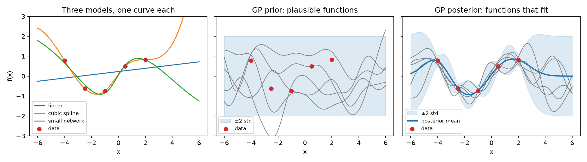
Consider fitting a curve through five observations of an unknown function. Linear regression, a spline, and a small neural network each give back a single curve (left panel). That curve is a best guess, but it does not say how far to trust it, either between the points or far away from them.
A Gaussian process (GP) keeps that uncertainty. Instead of committing to one function, it puts a probability distribution over functions.
- Before seeing data, the GP says which functions are plausible (middle panel).
- After seeing data, it gives more weight to the ones that agree with the observations and summarizes them as a mean curve with an error bar at every input (right panel).
- With Gaussian noise, both come in closed form.
Rasmussen and Williams (R&W) [1] state it formally:
A Gaussian process is a collection of random variables, any finite number of which have a joint Gaussian distribution.
Here the random variables are the function values f(x), one for each input x. So the definition says: pick any finite set of inputs, and the function values there are jointly Gaussian.
Two ideas turn this definition into a working regression method.
- A kernel sets the covariance between f(x) and f(x'). It decides which functions the GP finds plausible.
- Conditioning a Gaussian on the observed values turns the prior into the posterior.
So we start with kernels and the regression method they give on their own. Then we build the GP, fit its hyperparameters, and condition it on data. R&W [1] is the main reference for every GP result here.
Notation
- Inputs are x\in\mathbb{R}^d, and kernel arguments are written x,x'.
- The training set is x_1,\ldots,x_N with scalar labels y_1,\ldots,y_N.
- X\in\mathbb{R}^{N\times d} stacks the inputs as rows and y\in\mathbb{R}^N the labels.
- For a kernel k, the Gram matrix K=k(X,X)\in\mathbb{R}^{N\times N} has entries k(x_i,x_j).
- k(x,X)\in\mathbb{R}^{1\times N} is the row (k(x,x_1),\ldots,k(x,x_N)), and k(X,x) is its transpose.
- \varphi is a feature map.
From Kernels to Regression
What is a Kernel?
💡
In ML, a kernel is a measure of feature similarity based on a dot product.
Let's make this precise. A feature map \varphi:\mathbb{R}^d\to\mathbb{R}^D sends each input to a feature vector, and the kernel is the dot product of two feature vectors:
k(x,x')=\langle\varphi(x),\varphi(x')\rangle
With \varphi(x)=x, this is the standard dot product x^\top x' in the original space. A richer \varphi gives a richer notion of similarity: two inputs that look different in the original space can still be similar in feature space.
But a richer \varphi usually means a larger D, and building \varphi(x) gets expensive. Let's see with a small example. Take k(x,x')=(x^\top x')^2 and expand the square:
(x^\top x')^2=\sum_{i=1}^{d}\sum_{j=1}^{d}x_ix_j\,x'_ix'_j=\langle x\otimes x,\ x'\otimes x'\rangle
The matching feature map lists every pairwise product x_ix_j, so D=d^2 and the RHS dot product in feature space costs O(d^2). The LHS gives the same number for O(d): one dot product and a square.
Kernel trick: evaluate k directly and never build \varphi.
- The saving grows with D. For the radial basis function (RBF) kernel below, D is infinite, and the kernel trick is the only way to compute the similarity exactly.
Not every function of two inputs is a kernel. A symmetric function k is a kernel exactly when every Gram matrix K=k(X,X) it builds is positive semidefinite (PSD). We call k positive definite (PD) when these matrices are also invertible for distinct points. The toggle below has the details for readers who want the math.
Which Functions are Kernels?
A symmetric k is PSD if every Gram matrix is PSD:
\sum_{i=1}^{N}\sum_{j=1}^{N}\alpha_i\,\alpha_j\,k(x_i,x_j)\ \ge\ 0\qquad \forall N,\ \forall x_1,\ldots,x_N, \forall \alpha\in\mathbb{R}^N
A symmetric k is PD if the sum is strictly positive whenever \alpha\neq0 and the points are distinct. Note that naming varies: many texts call a PSD kernel "positive definite", and even [1] uses both names. This post keeps the matrix convention.
-
Every feature-map kernel is PSD.
- The quadratic form is \|\sum_i \alpha_i\varphi(x_i)\|^2\ge0.
-
Every PSD kernel is a feature-map kernel.
- The feature space may be infinite-dimensional, and there is a canonical choice: the reproducing kernel Hilbert space (RKHS) of k, explained in the next toggle [1].
- So "PSD" and "inner product of some features" are the same condition.
What is the RKHS?
For a PSD kernel k, there is a unique Hilbert space \mathcal{H} of functions that contains k(\cdot,x) for every input x and satisfies the reproducing property (Moore–Aronszajn):
f(x)=\langle f,\,k(\cdot,x)\rangle_{\mathcal{H}}\qquad\text{for every }f\in\mathcal{H}
The existence needs a proof, because an inner product cannot simply be declared. The construction starts from finite combinations f=\sum_i\alpha_i\,k(\cdot,x_i) and extends \langle k(\cdot,x),k(\cdot,x')\rangle_{\mathcal{H}}=k(x,x') bilinearly. Three checks make this an inner product:
-
Well-defined
- For g=\sum_j\beta_j k(\cdot,x'_j), \langle f,g\rangle_{\mathcal{H}}=\sum_j\beta_j f(x'_j)=\sum_i\alpha_i g(x_i), so it depends only on the values of f and g, not on how either is written.
-
Nonnegative
- \langle f,f\rangle_{\mathcal{H}}=\sum_{i,j}\alpha_i\alpha_j k(x_i,x_j)\ge0, which is exactly PSD.
-
Definite
- Cauchy–Schwarz, which needs only the nonnegativity above, gives f(x)^2\le\langle f,f\rangle_{\mathcal{H}}\,k(x,x), so \langle f,f\rangle_{\mathcal{H}}=0 forces f=0.
Finite combinations are not yet a Hilbert space, because a Hilbert space must be complete. So \mathcal{H} also takes in limits of finite combinations, such as f=\sum_{i=1}^{\infty}\alpha_i\,k(\cdot,x_i) whenever the partial sums form a Cauchy sequence in the \mathcal{H} -norm.
Two facts follow from the reproducing property:
-
The RKHS gives a feature map.
- Set f=k(\cdot,x') to get k(x,x')=\langle k(\cdot,x),k(\cdot,x')\rangle_{\mathcal{H}}, so \varphi(x)=k(\cdot,x) works for any PSD kernel. This proves the second bullet of the previous toggle.
-
Kernels and RKHSs match one to one, but kernels and feature maps do not.
- Each PSD kernel has exactly one RKHS (Moore–Aronszajn).
- The quadratic kernel above has many feature maps: x\otimes x\in\mathbb{R}^{d^2}, or a smaller one with x_i^2 and \sqrt{2}\,x_ix_j for i<j.
Examples
| kernel | k(x,x') | feature space |
|---|---|---|
| linear | x^\top x' | \varphi(x)=x, dimension d |
| polynomial | (\gamma\,x^\top x'+r)^q, \gamma>0, r>0, integer q\ge1 | all monomials of degree at most q, dimension \binom{d+q}{q} |
| RBF (squared exponential) | \exp\left(-\dfrac{\|x-x'\|^2}{2\ell^2}\right) | infinite-dimensional |
- In the RBF kernel, the length-scale \ell sets how far apart two inputs can be and still count as similar.
Why is RBF infinite-dimensional? Take d=1 and \ell=1. Split the square and expand the cross term as a power series:
e^{-(x-x')^2/2}=e^{-x^2/2}\,e^{-x'^2/2}\,e^{xx'}=\sum_{s=0}^{\infty}\left(\dfrac{e^{-x^2/2}\,x^s}{\sqrt{s!}}\right)\left(\dfrac{e^{-x'^2/2}\,x'^s}{\sqrt{s!}}\right)
The feature map has one coordinate for every power s, and no finite feature map gives the same kernel (proof in the toggle below). Yet evaluating the kernel costs one exponential.
Why Can't a Finite Feature Map Work?
-
Finite features cap the rank.
- For \varphi:\mathbb{R}^d\to\mathbb{R}^D, the Gram matrix is K=\Phi\Phi^\top with \Phi\in\mathbb{R}^{N\times D} stacking \varphi(x_i)^\top as rows, so \operatorname{rank}K\le D.
-
RBF Gram matrices have full rank.
- Write the RBF kernel as an average of waves. For \omega\sim\mathcal{N}(0,\ell^{-2}I), the characteristic function of a Gaussian gives \mathbb{E}_{\omega}\left[e^{i\omega^\top v}\right]=e^{-\|v\|^2/(2\ell^2)}, so with v=x-x', k(x,x')=\mathbb{E}_{\omega}\left[e^{i\omega^\top(x-x')}\right]. Hence
\alpha^\top K\alpha=\mathbb{E}_{\omega}\left[\Big|\sum_{j=1}^{N}\alpha_j\,e^{i\omega^\top x_j}\Big|^2\right]- The Gaussian density is positive everywhere, so this is 0 only if \sum_j \alpha_j e^{i\omega^\top x_j}=0 for every \omega. For distinct x_j these exponentials are linearly independent, so \alpha=0. Thus K is PD and invertible.
- So on D+1 distinct points, \operatorname{rank}K=D+1>D, and no D works.
Python Implementation and Result
The following code builds the Gram matrix of the RBF kernel on 20 random points in 2D and checks through its eigenvalues that it is PD.
-
Code Snippet
import numpy as np


def rbf(A, B, ell=1.0, sigma_f=1.0):
    """RBF kernel matrix k(A, B) for inputs of shape (n,) or (n, d)."""
    A, B = A.reshape(len(A), -1), B.reshape(len(B), -1)
    sq = ((A[:, None, :] - B[None, :, :]) ** 2).sum(-1)
    return sigma_f**2 * np.exp(-sq / (2 * ell**2))


rng = np.random.default_rng(0)
X = rng.uniform(-5, 5, size=(20, 2))  # 20 inputs in 2D
K = rbf(X, X, ell=1.0)

eigs = np.linalg.eigvalsh(K)  # symmetric, so real eigenvalues
print(f"symmetric: {np.allclose(K, K.T)}")
print(f"all eigenvalues positive: {bool((eigs > 0).all())}")
-
Result
symmetric: True
all eigenvalues positive: True
This matches the toggle above: on distinct points, the RBF Gram matrix is PD.
Kernel Ridge Regression
Kernel regression starts from a model that has no kernel in it yet. We model the target as a linear combination of features:
f(x)=\varphi(x)^\top w=\sum_{j=1}^{D}w_j\,\varphi_j(x),\qquad w\in\mathbb{R}^D
- The feature map \varphi is fixed in advance. It carries all the nonlinearity in x and decides which shapes f can take.
- Only the weights w are learned. Since f is linear in w, fitting stays a least-squares problem with a closed-form answer.
Let's fit w by ridge regression and rewrite the answer until only k is left.
Step 1: Weight Space
Stack the features as rows of \Phi\in\mathbb{R}^{N\times D}, row i being \varphi(x_i)^\top (R&W stack them as columns). Ridge regression minimizes the squared error plus a penalty on the weights, with \lambda>0:
J(w)=\|y-\Phi w\|^2+\lambda\|w\|^2
Set the gradient to zero:
\nabla_w J=-2\Phi^\top(y-\Phi w)+2\lambda w=0
\quad\Longrightarrow\quad
(\Phi^\top\Phi+\lambda I_D)\,w=\Phi^\top y
\Phi^\top\Phi is PSD, so \Phi^\top\Phi+\lambda I_D has eigenvalues at least \lambda and is invertible:
\hat w=(\Phi^\top\Phi+\lambda I_D)^{-1}\Phi^\top y
The formula needs a D\times D inverse. For the RBF kernel, D is infinite. So we need another route.
Step 2: Function Space
Step 1 ended with \hat w=(\Phi^\top\Phi+\lambda I_D)^{-1}\Phi^\top y, whose inverse is D\times D. We want the same \hat w with an N\times N inverse instead. The tool is a matrix identity, so let's derive it first. Note that
\Phi^\top(\Phi\Phi^\top+\lambda I_N)=\Phi^\top\Phi\Phi^\top+\lambda\Phi^\top=(\Phi^\top\Phi+\lambda I_D)\,\Phi^\top
Both bracketed matrices are invertible. Multiply on the left by (\Phi^\top\Phi+\lambda I_D)^{-1} and on the right by (\Phi\Phi^\top+\lambda I_N)^{-1} to get the identity we want:
(\Phi^\top\Phi+\lambda I_D)^{-1}\Phi^\top=\Phi^\top(\Phi\Phi^\top+\lambda I_N)^{-1}
Apply it to \hat w: then \hat w=\Phi^\top(\Phi\Phi^\top+\lambda I_N)^{-1}y, so the fitted weights are a combination of the training features \varphi(x_i). The prediction at a new input x is then
\hat f(x)=\varphi(x)^\top\hat w=\varphi(x)^\top\Phi^\top(\Phi\Phi^\top+\lambda I_N)^{-1}y
Now read off the two products:
- \varphi(x)^\top\Phi^\top is the row with entries \varphi(x)^\top\varphi(x_i)=k(x,x_i), which is k(x,X).
- \Phi\Phi^\top has entries \varphi(x_i)^\top\varphi(x_j)=k(x_i,x_j), which makes it the Gram matrix K.
Both products are kernel values, so this is where the kernel trick comes in: evaluate k directly, never build \varphi, and the features drop out:
\hat f(x)=k(x,X)\left(K+\lambda I\right)^{-1}y
This is kernel ridge regression (KRR). The cost is one N\times N solve, whatever D is. For an infinite-dimensional feature space, the same formula holds by the representer theorem, and the derivation above is its finite- D case [1].
💡
KRR predicts with
k(x, X)(K + λI)⁻¹y. Only the kernel appears, never the features.
Step 3: The Ridgeless Limit
What happens as the penalty vanishes? Let \lambda\to0 and assume K is invertible:
\hat f(x)=k(x,X)\,K^{-1}y=\sum_{i=1}^{N}\left(K^{-1}y\right)_i\,k(x_i,x)
The second form uses the symmetry k(x,x_i)=k(x_i,x).
-
The limit fits every training point exactly.
- At x=x_j, the row k(x_j,X) is row j of K. Times K^{-1}, that row gives the unit row e_j^\top, so \hat f(x_j)=y_j.
-
The limit is the minimum-norm fit.
- With an invertible K, \hat w=\Phi^\top(\Phi\Phi^\top)^{-1}y is the smallest-norm w that solves \Phi w=y.
This formula comes back later as the noiseless GP mean.
Gaussian Process Regression
KRR gives one function, with no sense of how far to trust it. A GP keeps the same kernel but puts a distribution over functions.
A Prior over Functions
A GP is a random function, written f\sim\mathcal{GP}(m,k). By the definition, its values on any finite set X are jointly Gaussian:
f(X)\sim\mathcal{N}\left(m(X),\ K\right),\qquad m(X)\in\mathbb{R}^N,\quad K=k(X,X)\in\mathbb{R}^{N\times N}
Two functions fill in this Gaussian on every finite set [1]:
- Mean function m, often set to zero. It gives the mean of each f(x).
- Covariance function k, the kernel. It gives the covariance between f(x) and f(x').
So building a GP means choosing m and k. Every computation with it then happens on a finite set.
Why must the kernel be PSD?
- K is a covariance matrix, so K must be PSD [1].
- Conversely, any mean function and any PSD kernel define a GP [1].
So the kernels from "What is a Kernel?" are exactly the valid covariance functions.
Nonparametric.
- A GP is an infinite-dimensional Gaussian, with one coordinate f(x) for every input x.
- Viewed as a Gaussian, its mean has an entry m(x) for every input and its covariance an entry k(x,x') for every pair of inputs, so it has infinitely many parameters.
- With an infinite-dimensional feature space, as for RBF, no finite weight vector can represent the GP. This is why GP regression is called nonparametric.
The kernel as a prior.
Choosing k is the main modeling assumption: it decides which functions are likely before any data arrive.
- The RBF kernel says nearby inputs have nearly equal outputs, and that the correlation decays over a distance \ell. A small \ell gives wiggly samples, a large \ell slowly varying ones.
- The linear kernel k(x,x')=x^\top x' gives linear functions f(x)=w^\top x, which are lines through the origin when d=1.
💡
So the choice of kernel strongly affects how well a GP predicts.
Python Implementation and Result
The following code draws five functions from \mathcal{GP}(0,k) with the RBF kernel, for \ell=0.2,\,1,\,5. On a grid X_* of 200 points in [-5,5], each is a draw of f(X_*)\sim\mathcal{N}\left(0,k(X_*,X_*)\right).
-
Code Snippet
import matplotlib.pyplot as plt
import numpy as np


def rbf(A, B, ell=1.0, sigma_f=1.0):
    """RBF kernel matrix k(A, B) for inputs of shape (n,) or (n, d)."""
    A, B = A.reshape(len(A), -1), B.reshape(len(B), -1)
    sq = ((A[:, None, :] - B[None, :, :]) ** 2).sum(-1)
    return sigma_f**2 * np.exp(-sq / (2 * ell**2))


rng = np.random.default_rng(0)
X_star = np.linspace(-5, 5, 200)
eps = 1e-6  # jitter for numerical stability

fig, axes = plt.subplots(1, 3, figsize=(12, 3.2), sharey=True)
for ax, ell in zip(axes, [0.2, 1.0, 5.0], strict=True):
    K_ss = rbf(X_star, X_star, ell=ell) + eps * np.eye(len(X_star))
    f = rng.multivariate_normal(np.zeros(len(X_star)), K_ss, size=5).T  # 5 draws
    ax.fill_between(X_star, -2, 2, color="gray", alpha=0.15, label="±2 std")
    ax.plot(X_star, f, lw=1.2)
    ax.set_title(f"ℓ = {ell}")
    ax.set_xlabel("x")

axes[0].set_ylabel("f(x)")
axes[0].legend(loc="lower left")
fig.tight_layout()
fig.savefig("gp_prior_samples.png", dpi=150)
-
Result
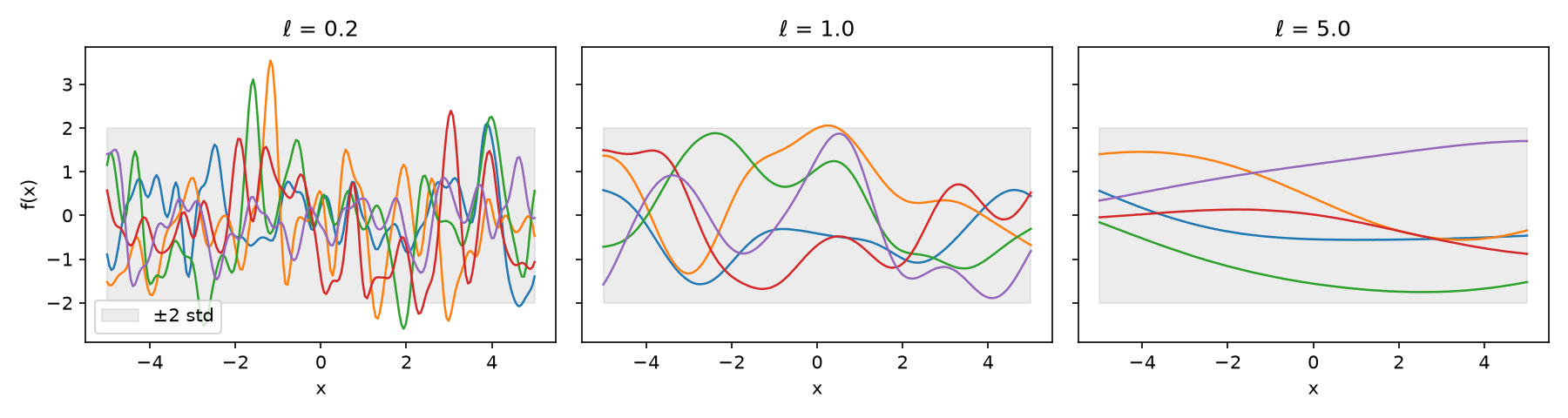
- Five samples from a zero-mean GP prior with an RBF kernel, for ℓ = 0.2, 1, 5. Smaller ℓ gives wigglier functions. The gray band is ±2 prior standard deviations.
The Model and Its Hyperparameters
The problem. We are given training data \mathcal{D}=(X,y), inputs x_1,\ldots,x_N with labels y_1,\ldots,y_N, and want to predict the unknown function at a new input x.
The model. Unlike KRR, there is no weight vector to fit. We model the function itself as random, and the labels as noisy readings of it:
- Prior: f\sim\mathcal{GP}(m,k), what we believe about f before any data.
- Likelihood: y_i=f(x_i)+\varepsilon_i with \varepsilon_i\sim\mathcal{N}(0,\sigma_n^2), how the labels arise from f. The noiseless case is \sigma_n=0.
The choices m, k and \sigma_n carry free constants, together called the hyperparameters \theta. For example, with a scalar input:
\begin{gathered}m(x)=ax^2+bx+c,\qquad k(x,x')=\sigma_f^2\exp\left(-\dfrac{(x-x')^2}{2\ell^2}\right),\\ \theta=[a,b,c,\sigma_f,\sigma_n,\ell]\end{gathered}
where \sigma_n^2 is the noise variance on the labels and \sigma_f^2 the signal variance.
Fitting them. Before predicting anything, we fit \theta to the data, and the GP itself supplies the objective. Under the model, f(X) is Gaussian and the noise is independent Gaussian, so their sum y is Gaussian too:
y\mid X,\theta\sim\mathcal{N}\left(m(X),\ K_y\right),\qquad K_y=K+\sigma_n^2I
So we fit \theta by minimizing the negative log marginal likelihood, the negative log of the Gaussian density of y with f integrated out [1]:
-\log p(y\mid X,\theta)=\dfrac{1}{2}\left(y-m(X)\right)^\top K_y^{-1}\left(y-m(X)\right)+\dfrac{1}{2}\log\det K_y+\dfrac{N}{2}\log 2\pi
The three terms have separate jobs [1].
- Data fit. The quadratic term is the only one that involves y. It measures how far y lies from m(X) in the metric given by K_y^{-1}.
- Complexity penalty. \log\det K_y is large for a flexible kernel, e.g. a short length-scale, that spreads probability over many datasets.
- Normalization. The last term does not depend on \theta.
Data fit against complexity acts as an automatic Occam's razor.
- Optimization: the gradient with respect to \theta is in closed form [1], so gradient descent or conjugate gradients apply.
- Cost: each step needs one Cholesky factorization of K_y, which is O(N^3). This cubic cost is the main limit of exact GPs [1].
Python Implementation and Result
The following code draws data from a GP with a known \theta, then checks that the marginal likelihood recovers it:
- True model. A cubic trend m(x)=1-0.8x+0.04x^3 plus a GP wiggle with \sigma_f=0.4 and \ell=0.5, observed with noise \sigma_n=0.1.
- Data. 80 labels on [-5,5]. The true f is drawn jointly with the data on a grid over [-6,6], so it can be plotted.
- Fit. A cubic mean m(x)=c_0+c_1x+c_2x^2+c_3x^3 with the RBF kernel above, so \theta=[c_0,c_1,c_2,c_3,\sigma_f,\sigma_n,\ell] has seven entries, all fitted by minimizing the negative log marginal likelihood.
- Plots. The left panel compares the true and fitted m(x). The right panel compares the posterior under the true and fitted \theta, using the formulas derived in "Conditioning on Data" below.
-
Code Snippet
import matplotlib.pyplot as plt
import numpy as np
from scipy.optimize import minimize


def rbf(A, B, ell=1.0, sigma_f=1.0):
    """RBF kernel matrix k(A, B) for inputs of shape (n,) or (n, d)."""
    A, B = A.reshape(len(A), -1), B.reshape(len(B), -1)
    sq = ((A[:, None, :] - B[None, :, :]) ** 2).sum(-1)
    return sigma_f**2 * np.exp(-sq / (2 * ell**2))


def mean_fn(x, coef):
    """Cubic mean m(x) = c0 + c1 x + c2 x² + c3 x³."""
    return np.polyval(coef[::-1], x)


# True model: a cubic trend m plus a short-wavelength GP wiggle, labels y = f(x) + noise
rng = np.random.default_rng(0)
coef_true = np.array([1.0, -0.8, 0.0, 0.04])  # c0, c1, c2, c3
sigma_f, sigma_n, ell = 0.4, 0.1, 0.5  # true kernel and noise hyperparameters
N = 80
X = np.sort(rng.uniform(-5, 5, N))
xs = np.linspace(-6, 6, 300)
Z = np.concatenate([X, xs])  # draw the GP part at the data and on a grid together
g = rng.multivariate_normal(np.zeros(len(Z)), rbf(Z, Z, ell, sigma_f) + 1e-8 * np.eye(len(Z)))
f_xs = mean_fn(xs, coef_true) + g[N:]  # true f on the grid
y = mean_fn(X, coef_true) + g[:N] + sigma_n * rng.standard_normal(N)


def nlml(theta):
    """-log p(y | X, θ), with σ_f, σ_n, ℓ passed as logs to keep them positive."""
    coef, (log_sf, log_sn, log_ell) = theta[:4], theta[4:]
    r = y - mean_fn(X, coef)  # y - m(X)
    K_y = rbf(X, X, np.exp(log_ell), np.exp(log_sf)) + np.exp(2 * log_sn) * np.eye(N)
    L = np.linalg.cholesky(K_y)
    alpha = np.linalg.solve(L.T, np.linalg.solve(L, r))
    log_det = 2 * np.log(np.diag(L)).sum()  # log det K_y
    return 0.5 * r @ alpha + 0.5 * log_det + 0.5 * N * np.log(2 * np.pi)


res = minimize(nlml, x0=np.zeros(7), method="L-BFGS-B")
coef_ = res.x[:4]
sf_, sn_, ell_ = np.exp(res.x[4:])


def posterior(xs, coef, sigma_f, sigma_n, ell):
    """Posterior mean and std of f at xs, from "Conditioning on Data"."""
    K_y = rbf(X, X, ell, sigma_f) + sigma_n**2 * np.eye(N)
    K_s = rbf(xs, X, ell, sigma_f)  # k(x, X)
    mean = mean_fn(xs, coef) + K_s @ np.linalg.solve(K_y, y - mean_fn(X, coef))
    cov = rbf(xs, xs, ell, sigma_f) - K_s @ np.linalg.solve(K_y, K_s.T)
    return mean, np.sqrt(np.clip(np.diag(cov), 0, None))


fig, axes = plt.subplots(1, 2, figsize=(12, 3.8))
axes[0].scatter(X, y, s=10, c="C3", zorder=3, label="data")
axes[0].plot(xs, mean_fn(xs, coef_true), "k--", label="true m(x)")
axes[0].plot(xs, mean_fn(xs, coef_), "C0", label="fitted m(x)")
axes[0].set_title(f"fitted σ_f = {sf_:.2f}, σ_n = {sn_:.2f}, ℓ = {ell_:.2f}")

axes[1].plot(xs, f_xs, "k", lw=1, label="true f(x)")
mean, std = posterior(xs, coef_, sf_, sn_, ell_)  # fitted θ: filled band
axes[1].plot(xs, mean, "C0", label="posterior mean, fitted θ")
axes[1].fill_between(xs, mean - 2 * std, mean + 2 * std, color="C0", alpha=0.2,
                     label="±2 std, fitted θ")
mean, std = posterior(xs, coef_true, sigma_f, sigma_n, ell)  # true θ: band edges only
axes[1].plot(xs, mean, "C1--", label="posterior mean, true θ")
axes[1].plot(xs, mean - 2 * std, "C1:", lw=1, label="±2 std, true θ")
axes[1].plot(xs, mean + 2 * std, "C1:", lw=1)
axes[1].scatter(X, y, s=10, c="C3", zorder=3, label="data")
axes[1].axvspan(-6, -5, color="gray", alpha=0.08)
axes[1].axvspan(5, 6, color="gray", alpha=0.08)  # no data here
axes[1].set_title("posterior of f under the true and fitted θ")
for ax in axes:
    ax.set_xlabel("x")
    ax.legend(fontsize=7)
fig.tight_layout()
fig.savefig("gp_nlml_fit.png", dpi=150)
-
Result
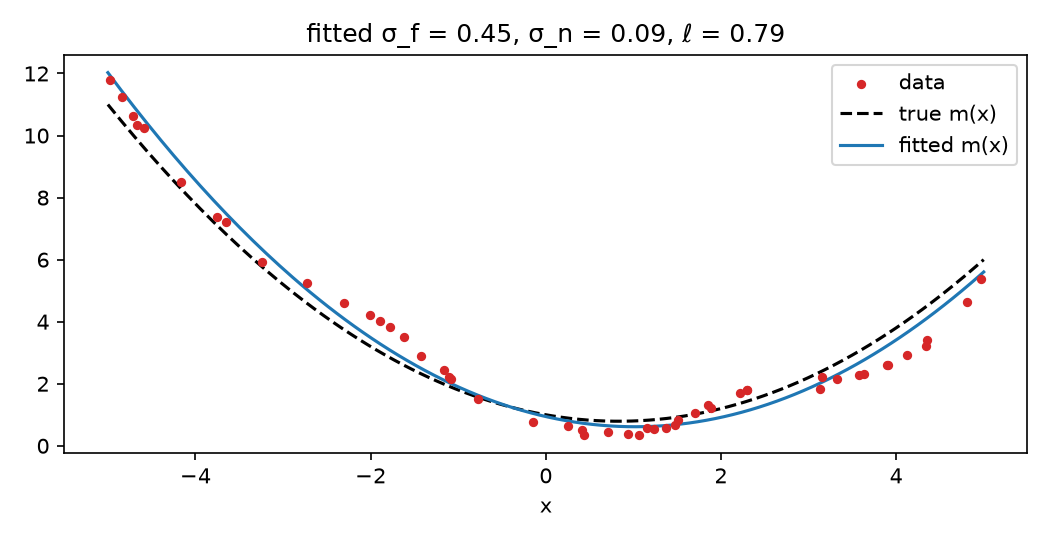
- Left: the fitted cubic lands close to the true trend (within about 0.3), and the kernel hyperparameters come back close to their true values ( \sigma_f=0.39 vs 0.4, \sigma_n=0.11 vs 0.1, \ell=0.51 vs 0.5).
- Right: inside the data range, the posteriors under the true and the fitted \theta nearly coincide and follow the true f with a narrow band. In the shaded regions with no data, both bands widen.
Conditioning on Data
With \theta fitted, we can now predict with the posterior p(f(x)\mid\mathcal{D}): its mean is the prediction, and its variance is the error bar. Bayes' rule gives p(f\mid\mathcal{D})\propto p(y\mid f)\,p(f), which usually has no closed form. Here everything is jointly Gaussian, so the posterior is a conditional Gaussian.
Conditioning a Gaussian
Split a jointly Gaussian vector into two blocks:
\begin{bmatrix}z_1\\ z_2\end{bmatrix}\sim\mathcal{N}\left(\begin{bmatrix}\mu_1\\ \mu_2\end{bmatrix},\begin{bmatrix}\Sigma_{11}&\Sigma_{12}\\ \Sigma_{21}&\Sigma_{22}\end{bmatrix}\right)
Assuming \Sigma_{11} is invertible, the conditional of z_2 given z_1 is Gaussian [1]:
\begin{aligned}
z_2\mid z_1&\sim\mathcal{N}\left(\mu_{2|1},\ \Sigma_{2|1}\right)\\
\mu_{2|1}&=\mu_2+\Sigma_{21}\Sigma_{11}^{-1}(z_1-\mu_1)\\
\Sigma_{2|1}&=\Sigma_{22}-\Sigma_{21}\Sigma_{11}^{-1}\Sigma_{12}
\end{aligned}
What's the meaning of this?
- The mean shifts by the observed surprise z_1-\mu_1, weighted by \Sigma_{21}\Sigma_{11}^{-1}: the cross-covariance scaled by the inverse covariance of z_1.
- The covariance shrinks by an amount that does not depend on the observed values.
Noiseless Observations
Suppose we observe f(X)=y exactly, and assume K is invertible, as for a PD kernel on distinct inputs. By the finite-set property, the training values and the value at a test input x are jointly Gaussian:
\begin{bmatrix}f(X)\\ f(x)\end{bmatrix}\sim\mathcal{N}\left(\begin{bmatrix}m(X)\\ m(x)\end{bmatrix},\begin{bmatrix}K&k(X,x)\\ k(x,X)&k(x,x)\end{bmatrix}\right)
Match the blocks to the conditioning formula:
- z_1=f(X), observed as y, and z_2=f(x).
- \mu_1=m(X) and \mu_2=m(x).
- \Sigma_{11}=K, \Sigma_{21}=k(x,X) and \Sigma_{22}=k(x,x).
Plugging in gives the posterior at x. Replacing the single test input by any finite set of test inputs gives the same formulas blockwise, so every finite set is jointly Gaussian after conditioning and the posterior is again a GP, f\mid\mathcal{D}\sim\mathcal{GP}(m_{\mathcal{D}},k_{\mathcal{D}}), with \mathcal{D}=(X,y) and
\begin{aligned}
m_{\mathcal{D}}(x)&=m(x)+k(x,X)\,K^{-1}\left(y-m(X)\right)\\
k_{\mathcal{D}}(x,x')&=k(x,x')-k(x,X)\,K^{-1}\,k(X,x')
\end{aligned}
Noisy Observations
With noise we observe y instead of f(X), so the first block becomes y:
\begin{bmatrix}y\\ f(x)\end{bmatrix}\sim\mathcal{N}\left(\begin{bmatrix}m(X)\\ m(x)\end{bmatrix},\begin{bmatrix}K+\sigma_n^2I&k(X,x)\\ k(x,X)&k(x,x)\end{bmatrix}\right)
Only the top-left block changes: independent noise adds to the diagonal and leaves the cross terms alone. Plugging in again gives [1]:
\begin{aligned}
m_{\mathcal{D}}(x)&=m(x)+k(x,X)\left(K+\sigma_n^2I\right)^{-1}\left(y-m(X)\right)\\
k_{\mathcal{D}}(x,x')&=k(x,x')-k(x,X)\left(K+\sigma_n^2I\right)^{-1}k(X,x')
\end{aligned}
So noise does one thing: it replaces K by K+\sigma_n^2I. To predict a new noisy label rather than f(x), add \sigma_n^2 to the variance k_{\mathcal{D}}(x,x).
What does noise change at a training point?
| Noiseless ( \sigma_n^2=0 ) | Noisy ( \sigma_n^2>0 ) | |
|---|---|---|
| posterior mean m_{\mathcal{D}}(x_i) | =y_i (interpolation) | pulled off y_i (regression) |
| posterior variance k_{\mathcal{D}}(x_i,x_i) | =0 at the training inputs (for RBF, positive elsewhere) | >0 (residual uncertainty) |
| role | interpolator | smoother, denoiser |
Derivation
Assume K is PD.
- Noiseless: k(x_i,X)K^{-1}=e_i^\top, so m_{\mathcal{D}}(x_i)=y_i and k_{\mathcal{D}}(x_i,x_i)=k(x_i,x_i)-k(x_i,x_i)=0.
- Noisy, means: on the training set m_{\mathcal{D}}(X)-m(X)=K(K+\sigma_n^2I)^{-1}(y-m(X)). In the eigenbasis of K, with eigenvalues \nu_j, each component of the residual y-m(X) is multiplied by \nu_j/(\nu_j+\sigma_n^2)<1. The shrinkage acts on eigendirections, not on points: a single posterior mean can land farther from the prior mean than its label.
- Noisy, variances: K-K(K+\sigma_n^2I)^{-1}K=K(K+\sigma_n^2I)^{-1}\left[(K+\sigma_n^2I)-K\right]=\sigma_n^2K(K+\sigma_n^2I)^{-1}. This matrix is PD, so each diagonal entry is positive.
Python Implementation and Result
The following code plugs eight points of \sin(x) into the posterior formulas above, noiseless and noisy side by side. It uses m=0, the RBF kernel with \ell=1 and \sigma_f=1, and \sigma_n=0 and 0.3 set by hand.
-
Code Snippet
import matplotlib.pyplot as plt
import numpy as np


def rbf(A, B, ell=1.0, sigma_f=1.0):
    """RBF kernel matrix k(A, B) for inputs of shape (n,) or (n, d)."""
    A, B = A.reshape(len(A), -1), B.reshape(len(B), -1)
    sq = ((A[:, None, :] - B[None, :, :]) ** 2).sum(-1)
    return sigma_f**2 * np.exp(-sq / (2 * ell**2))


def gp_posterior(X, y, X_star, sigma_n, ell=1.0, jitter=1e-10):
    """Posterior mean and std at X_star, with zero prior mean."""
    K_y = rbf(X, X, ell) + (sigma_n**2 + jitter) * np.eye(len(X))  # K + σ_n² I
    K_s = rbf(X_star, X, ell)  # k(x, X), one row per test input
    mean = K_s @ np.linalg.solve(K_y, y)  # m_D(x)
    cov = rbf(X_star, X_star, ell) - K_s @ np.linalg.solve(K_y, K_s.T)  # k_D(x, x')
    return mean, np.sqrt(np.clip(np.diag(cov), 0, None))


rng = np.random.default_rng(1)
X = rng.uniform(-4.5, 4.5, 8)
X_star = np.linspace(-5, 5, 200)


fig, axes = plt.subplots(1, 2, figsize=(11, 3.6), sharey=True)
for ax, sigma_n in zip(axes, [0.0, 0.3], strict=True):
    y = np.sin(X) + sigma_n * rng.standard_normal(len(X))
    mean, std = gp_posterior(X, y, X_star, sigma_n)
    ax.plot(X_star, np.sin(X_star), "k--", lw=1, label="sin(x)")
    ax.plot(X_star, mean, "C0", label="posterior mean")
    ax.fill_between(
        X_star, mean - 2 * std, mean + 2 * std, color="C0", alpha=0.2, label="±2 std"
    )
    ax.scatter(X, y, c="C3", zorder=3, label="training points")
    ax.set_title(f"σ_n = {sigma_n}")
    ax.set_xlabel("x")

axes[0].set_ylabel("f(x)")
axes[0].legend(loc="lower left", fontsize=8)
fig.tight_layout()
fig.savefig("gp_posterior.png", dpi=150)
-
Result
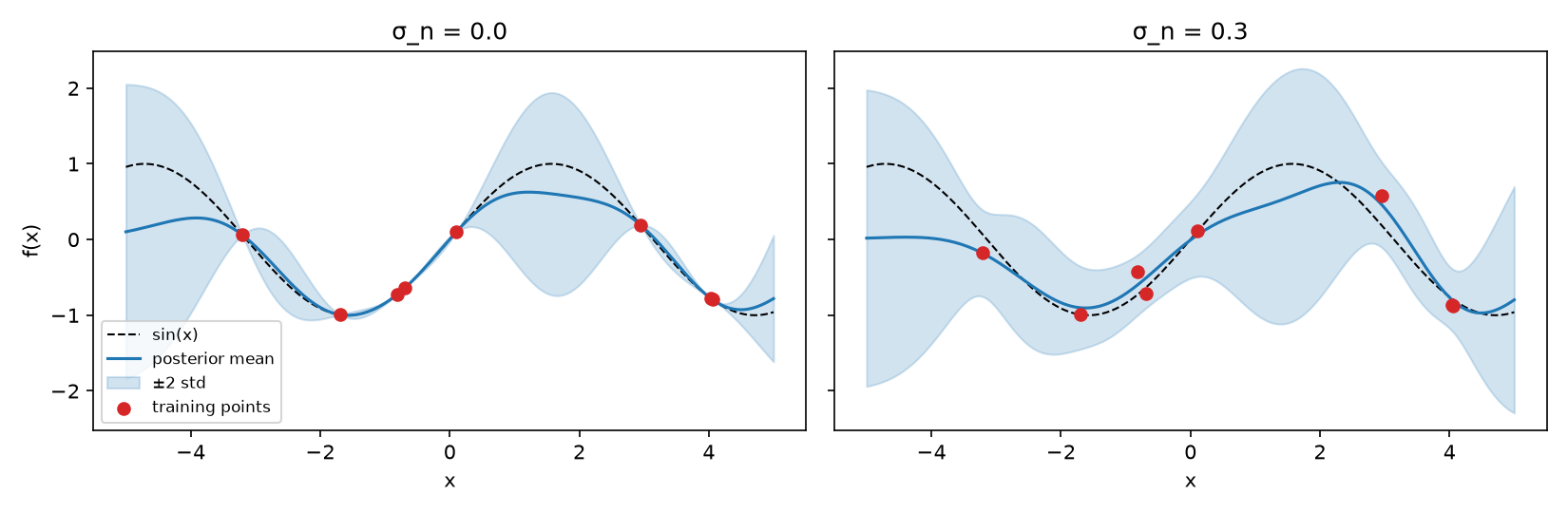
- GP posterior from eight points of \sin(x), RBF kernel with ℓ = 1. Left: noiseless labels. Right: noise with σ_n = 0.3.
- Without noise, the band pinches to zero at the points. With noise, it stays open.
How Are Kernel Regression and GP Related?
The GP Mean is Kernel Ridge Regression
Let's put the two mean formulas side by side, with a zero prior mean:
\begin{aligned}
\text{KRR:}&\quad \hat f(x)=k(x,X)\left(K+\lambda I\right)^{-1}y\\
\text{GP, noise }\sigma_n^2:&\quad m_{\mathcal{D}}(x)=k(x,X)\left(K+\sigma_n^2I\right)^{-1}y
\end{aligned}
The two formulas are the same expression with \lambda=\sigma_n^2 [1]. In the noiseless case, \sigma_n^2=0 with K invertible, the GP mean is the ridgeless formula k(x,X)\,K^{-1}y.
Why is the match exact?
For a finite feature dimension D, the ridge penalty is a Gaussian prior on the weights in disguise: with w\sim\mathcal{N}(0,I_D) and noise variance \sigma_n^2=\lambda, the ridge solution is the posterior mean of w. "The Weight-Space View" below proves this in full.
- KRR returns one function. \lambda is a regularization strength.
- GP regression returns a distribution. Its mean is the KRR function, and \sigma_n^2 is a noise level.
💡
The GP posterior mean with noise variance
σ_n²
is KRR with
λ = σ_n². What the GP adds is the posterior variance.
Python Implementation and Result
The following code fits KRR with \lambda=\sigma_n^2 and the GP on the same 30 noisy points of \sin(x). Both use the RBF kernel with \ell=1 and \sigma_f=1, and \sigma_n=0.3. The GP takes m=0.
-
Code Snippet
import matplotlib.pyplot as plt
import numpy as np


def rbf(A, B, ell=1.0, sigma_f=1.0):
    """RBF kernel matrix k(A, B) for inputs of shape (n,) or (n, d)."""
    A, B = A.reshape(len(A), -1), B.reshape(len(B), -1)
    sq = ((A[:, None, :] - B[None, :, :]) ** 2).sum(-1)
    return sigma_f**2 * np.exp(-sq / (2 * ell**2))


rng = np.random.default_rng(2)
sigma_n = 0.3
X = rng.uniform(-5, 5, 30)
y = np.sin(X) + sigma_n * rng.standard_normal(30)
X_star = np.linspace(-5, 5, 200)
K, K_s = rbf(X, X), rbf(X_star, X)  # K and k(x, X)

# Kernel ridge regression with λ = σ_n²
lam = sigma_n**2
f_krr = K_s @ np.linalg.solve(K + lam * np.eye(len(X)), y)

# GP posterior mean and std
K_y = K + sigma_n**2 * np.eye(len(X))
m_gp = K_s @ np.linalg.solve(K_y, y)
cov = rbf(X_star, X_star) - K_s @ np.linalg.solve(K_y, K_s.T)
std = np.sqrt(np.clip(np.diag(cov), 0, None))

fig, ax = plt.subplots(figsize=(7, 3.6))
ax.fill_between(
    X_star, m_gp - 2 * std, m_gp + 2 * std, color="C0", alpha=0.2, label="GP ±2 std"
)
ax.plot(X_star, m_gp, "C0", lw=4, alpha=0.5, label="GP posterior mean")
ax.plot(X_star, f_krr, "k--", lw=1.2, label="KRR, λ = σ_n²")
ax.scatter(X, y, s=14, c="C3", zorder=3, label="data")
ax.set_xlabel("x")
ax.legend(loc="lower left", fontsize=8)
fig.tight_layout()
fig.savefig("gp_krr.png", dpi=150)
-
Result
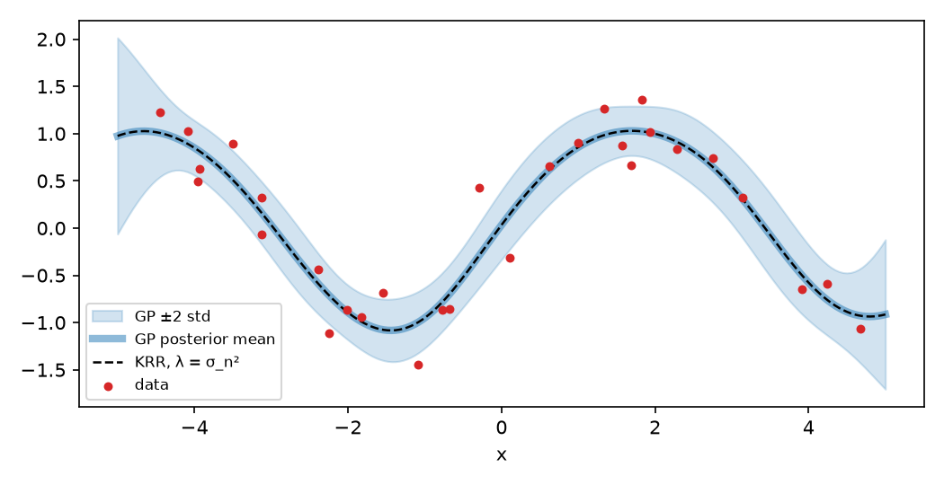
- KRR (dashed) lies exactly on the GP posterior mean. Only the GP adds the ±2 std band.
Which "kernel regression"?
In statistics, the phrase often means the Nadaraya–Watson estimator [3,4], a local average of the labels with nonnegative kernel weights. That is a different method: the GP mean equals KRR, not Nadaraya–Watson.
The Weight-Space View
So far the GP lives in function space: a distribution placed directly on f. The same model has a weight-space form, where the randomness sits in the weights of a linear model [1].
- Both describe the same model. They differ in what is treated as random:
| Weight space | Function space | |
|---|---|---|
| random object | weights w\in\mathbb{R}^D | function values f(x) |
| prior | w\sim\mathcal{N}(0,\Sigma_p) | f\sim\mathcal{GP}(m,k) |
| modeling choice | features \varphi and \Sigma_p | kernel k |
| posterior needs | a D\times D inverse | an N\times N inverse |
| works when | D is finite | any PSD kernel, even infinite D |
Bayesian Linear Regression is a GP
Start from the KRR model f(x)=\varphi(x)^\top w. Ridge regression picks one best w. Bayesian linear regression instead treats w as random: it puts a prior w\sim\mathcal{N}(0,\Sigma_p) on the weights, with \Sigma_p\in\mathbb{R}^{D\times D} positive definite, and updates it with the data by Bayes' rule. The prior on w is what makes it Bayesian.
A random w makes f a random function, and in fact a GP:
- It is a GP. On any finite set of inputs, f(X)=\Phi w is a linear map of a Gaussian vector, so it is Gaussian. That is exactly the GP definition.
-
Its mean and kernel.
- The mean is \mathbb{E}[f(x)]=\varphi(x)^\top\mathbb{E}[w]=0.
-
And the covariance is
\mathbb{E}\left[f(x)f(x')\right]=\mathbb{E}\left[\varphi(x)^\top w\,w^\top\varphi(x')\right]=\varphi(x)^\top\,\mathbb{E}[ww^\top]\,\varphi(x')=\varphi(x)^\top\Sigma_p\,\varphi(x')
So a Gaussian prior on w is the same thing as the GP prior f\sim\mathcal{GP}(0,k) with k(x,x')=\varphi(x)^\top\Sigma_p\,\varphi(x') [1]. With \Sigma_p=I this is the feature-map kernel from "What is a Kernel?".
The next question is whether updating w with data gives the same posterior as conditioning the GP.
Do the Two Posteriors Agree?
Yes. With noise of variance \sigma_n^2>0, the weight-space predictive mean and covariance are exactly m_{\mathcal{D}} and k_{\mathcal{D}} from "Conditioning on Data", with m=0 and k(x,x')=\varphi(x)^\top\Sigma_p\varphi(x') [1]. The toggle below has the derivation.
Derivation
Step 1: Posterior over weights. By Bayes' rule, the log posterior over w is the log likelihood plus the log prior:
\log p(w\mid X,y)=-\dfrac{1}{2\sigma_n^2}\|y-\Phi w\|^2-\dfrac{1}{2}w^\top\Sigma_p^{-1}w+\text{const}
Collect the terms in w, with A=\sigma_n^{-2}\Phi^\top\Phi+\Sigma_p^{-1}:
\log p(w\mid X,y)=-\dfrac{1}{2}w^\top A\,w+\sigma_n^{-2}w^\top\Phi^\top y+\text{const}=-\dfrac{1}{2}(w-\bar w)^\top A\,(w-\bar w)+\text{const}
where \bar w=\sigma_n^{-2}A^{-1}\Phi^\top y. So w\mid X,y\sim\mathcal{N}(\bar w,A^{-1}).
Step 2: Predictive mean. The predictive mean at x is \varphi(x)^\top\bar w. We turn it into kernel form with the same identity trick as in KRR. Note that
A\,\Sigma_p\Phi^\top=\sigma_n^{-2}\Phi^\top\Phi\Sigma_p\Phi^\top+\Phi^\top=\sigma_n^{-2}\Phi^\top\left(\Phi\Sigma_p\Phi^\top+\sigma_n^2I\right)
Multiply on the left by A^{-1} and on the right by (\Phi\Sigma_p\Phi^\top+\sigma_n^2I)^{-1}:
\Sigma_p\Phi^\top\left(\Phi\Sigma_p\Phi^\top+\sigma_n^2I\right)^{-1}=\sigma_n^{-2}A^{-1}\Phi^\top
Now \Phi\Sigma_p\Phi^\top=K and \varphi(x)^\top\Sigma_p\Phi^\top=k(x,X). Hence
\varphi(x)^\top\bar w=k(x,X)\left(K+\sigma_n^2I\right)^{-1}y
That is exactly the function-space posterior mean.
Step 3: Predictive variance. The Woodbury identity with A=\Sigma_p^{-1}+\Phi^\top(\sigma_n^2I)^{-1}\Phi gives
A^{-1}=\Sigma_p-\Sigma_p\Phi^\top\left(\Phi\Sigma_p\Phi^\top+\sigma_n^2I\right)^{-1}\Phi\Sigma_p
so \varphi(x)^\top A^{-1}\varphi(x')=k(x,x')-k(x,X)(K+\sigma_n^2I)^{-1}k(X,x'), which is k_{\mathcal{D}}(x,x').
💡
Bayesian linear regression on features
φ
with prior covariance
Σₚ
is the GP with kernel
φ(x)ᵀΣₚφ(x'). Weights and functions are two views of one model.
Next Steps
-
The posterior variance is what makes GPs useful beyond regression.
- Bayesian optimization uses it to choose the next point to evaluate: where the mean looks promising or the error bar is still wide.
- For practical treatments with code, see the Dive into Deep Learning chapter [2] and Roelants' tutorial [5].
Reference
[1] Rasmussen, C. E., & Williams, C. K. I. (2006). Gaussian Processes for Machine Learning. MIT Press.
http://gaussianprocess.org/gpml/
[2] Zhang, A., Lipton, Z. C., Li, M., & Smola, A. J. Dive into Deep Learning, ch. 18 "Gaussian Processes".
https://d2l.ai/chapter_gaussian-processes/index.html
[3] Nadaraya, E. A. (1964). On Estimating Regression. Theory of Probability and Its Applications, 9(1), 141–142.
https://doi.org/10.1137/1109020
[4] Watson, G. S. (1964). Smooth Regression Analysis. Sankhyā: The Indian Journal of Statistics, Series A, 26(4), 359–372.
https://www.jstor.org/stable/25049340
[5] Roelants, P. (2019). Gaussian processes (1/3) - From scratch.
https://peterroelants.github.io/posts/gaussian-process-tutorial/