Supplement to: Neural Solver Towards Future of Simulation: Intro

• Having explored the potential of Neural Solvers in my previous post, we now return to the 'classic' foundations of CFD(Computational Fluid Dynamics) to clearly define the core problems that neural solvers are actually trying to solve.

• Prepared for a Deepest seminar, this guide introduces FDM and FEM to bridge the gap between traditional CFD logic and neural solver goals.

• The following sections break down the mathematical discretization of the governing equations. Python implementations are provided to run and visualize these systems in action.

The Challenge: From Calculus to Computation

• The physical world is governed by Differential Equations (DEs) , which describe how continuous quantities such as temperature, pressure, or velocity change across space and time.

• Computers cannot solve differential equations analytically in their continuous form; they require numerical discretization to translate continuous calculus into discrete machine arithmetic.

• Discretization bridges this gap by breaking a continuous domain into small, solvable chunks. The specific strategy chosen to partition the domain defines the resulting method: the Grid Approach (FDM) or the Mesh Approach (FEM).

Finite Difference Method (FDM): The Grid Approach

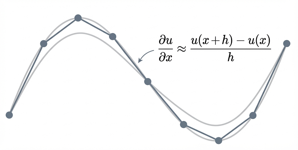
FDM is the most intuitive method. It approximates derivatives as the slope between neighbors , provided the function is smooth enough for discrete differences to mimic continuous change.

The Problem: 1D Heat Equation

Let’s start with the classic 1D Heat Equation. This simulates how temperature diffuses through a thin metal rod over time.

• u(x,t) : Temperature at position x and time t .

• LHS ( \dfrac{\partial u}{\partial t} ) : The rate of temperature change at a specific point.

• RHS ( \dfrac{\partial^2 u}{\partial x^2} ) : The curvature of the distribution.

• Physics : Heat flows to smooth out this curvature until equilibrium is reached.

Physical Environment:

Establishing the simulation requires a defined physical domain and initial state.

• Domain : A rod of length L=1 located on the interval [0, 1] .

• Boundary Conditions (BCs) : Both ends are fixed at zero heat, known as a Dirichlet BC.

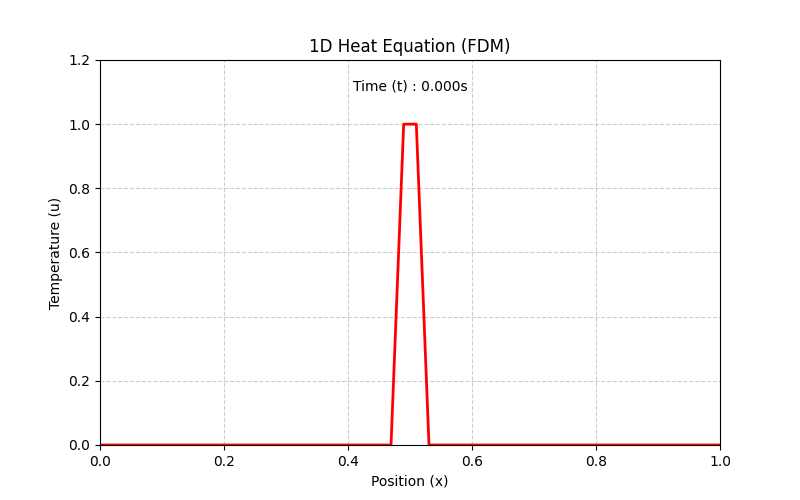
• Initial State & Event : The rod starts with zero heat everywhere ($u=0$), but a sudden heat spike is applied to the center.

• Initial Condition (IC) : The rod is at zero heat everywhere, except for that sudden heat spike in the center at t=0 .

  

Step-by-Step: Turning Physics into Code

Converting the continuous PDE into a computable form relies on approximating derivatives using discrete grid points. A grid is established where u_i^n represents the temperature at position i and time step n .

Step 1: Discretize Time (Forward Difference)

The rate of change over time is approximated by the difference between the current state n and the future state n+1 :

Step 2: Discretize Space (Central Difference)

The curvature (2nd derivative) at grid point i is approximated using the values of its immediate neighbors, i-1 and i+1 :

Step 3: The Update Rule

Substituting these discrete approximations back into the original heat equation:

Isolating the future state u_i^{n+1} yields the final algebraic formula used in the simulation logic:

where r = \dfrac{\alpha \Delta t}{\Delta x^2} remains constant throughout the execution.

Python Implementation and Result

The following implementation simulates the 1D Heat Equation system and generates a visualized GIF of the results.

• Code Snippet

  import numpy as np
  import matplotlib.pyplot as plt
  from matplotlib.animation import FuncAnimation, PillowWriter
  
  
  # --- 1. Configuration & Physics Setup ---
  L = 1.0
  nx = 50
  dx = L / (nx - 1)
  alpha = 0.01
  dt = 0.0005
  t_final = 1.2
  steps_per_frame = 100
  frames = int(t_final / (steps_per_frame * dt))
  
  x = np.linspace(0, L, nx)
  r = alpha * dt / (dx**2)
  
  # Initial Condition
  u = np.zeros(nx)
  mid = int(nx / 2)
  u[mid - 1 : mid + 1] = 1.0
  
  # --- 2. Run Simulation ---
  print("Running FDM Simulation...")
  history = [u.copy()]  # Store t=0
  current_u = u.copy()
  
  for frame in range(frames):
      for _ in range(steps_per_frame):
          # Update Rule
          current_u[1:-1] = current_u[1:-1] + r * (
              current_u[2:] - 2 * current_u[1:-1] + current_u[:-2]
          )
      history.append(current_u.copy())
  print("Simulation Complete.")
  
  # --- 3. Visualization & Saving ---
  fig, ax = plt.subplots(figsize=(8, 5))
  (line,) = ax.plot(x, history[0], color="red", linewidth=2, label="Temperature")
  
  ax.set_xlim(0, L)
  ax.set_ylim(0, 1.2)
  ax.set_xlabel("Position (x)")
  ax.set_ylabel("Temperature (u)")
  ax.grid(True, linestyle="--", alpha=0.6)
  title = ax.set_title("1D Heat Equation (FDM)")
  subtitle = ax.text(
      0.5, 0.95, "Time (t) : 0.000s", transform=ax.transAxes, ha="center", va="top"
  )
  
  
  def update(frame):
      u_state = history[frame]
      line.set_ydata(u_state)
      title.set_text("1D Heat Equation (FDM)")
      subtitle.set_text(f"Time (t) : {frame * steps_per_frame * dt:.3f}s")
      return line, title
  
  
  ani = FuncAnimation(fig, update, frames=len(history), interval=25, blit=True)
  
  # --- 4. Save GIF ---
  print("Saving GIF...")
  writer = PillowWriter(fps=15)
  ani.save("heat_fdm.gif", writer=writer)
  print("Saved to heat_fdm.gif")
  

• Result

  

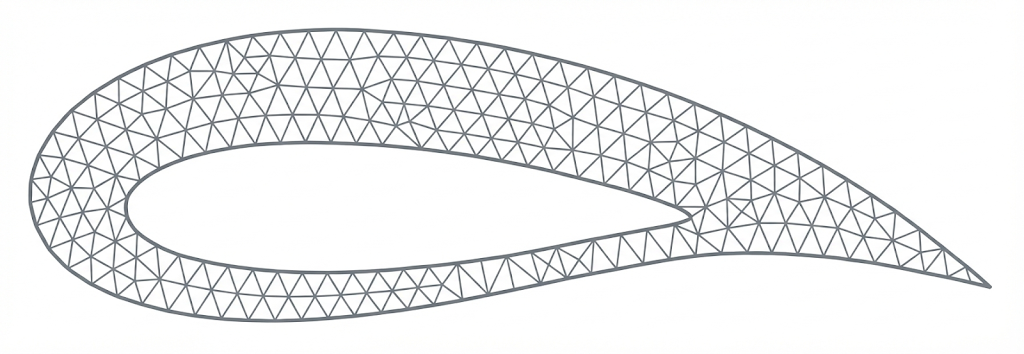
Finite Element Method (FEM): The Mesh Approach

Complex geometries, such as airplane wings, require more flexibility than rigid grids that rigid grids cannot provide. The FEM addresses this by partitioning the domain into unstructured elements.

• These flexible shapes allow the simulation to conform to curved boundaries and irregular holes with high precision.

While distinct in application, FEM and FDM are complementary tools in the CFD pipeline.

• The choice between a grid-based or mesh-based approach depends strictly on the geometric requirements of the simulation.

The Problem: 2D Wave Equation

Beyond static diffusion, the 2D Wave Equation simulates how physical disturbances, such as water ripples, propagate through a two-dimensional domain:

• u(x,y,t) : The vertical displacement (height) of the water surface at position (x,y) and time t .

• c : The wave speed.

• LHS ( \dfrac{\partial^2 u}{\partial t^2} ) : Vertical Acceleration. Tracks the rate of change in vertical velocity at a specific point.

• RHS ( \nabla^2 u ) : The Restoring Force. The Laplacian measures the local average difference, acting as the restoring force that pulls the surface toward equilibrium.

• Physics : The system constantly drives toward equilibrium. A peak (convex) is pulled down, and a trough (concave) is pushed up, creating the ripple effect.

Case 1: No Obstacle

Physical Environment:

• Domain : A square pool defined by x \in [-1, 1] and y \in [-1, 1] .

• Boundary Conditions : Four outer walls fixed at height 0 (Dirichlet BC).

• Mesh : Delaunay triangulation of a square grid.

• Initial Condition : Flat water surface ( u=0 ) with a Gaussian droplet peak at [0.5, 0.5] .

Step-by-Step: Turning Physics into Code

To simulate the water drop, the continuous wave equation is converted into a system of discrete matrix algebra solved iteratively in Python.

• Step 1: The Weak Formulation (FEM Setup)

  To apply FEM, the equation is multiplied by a test function v and integrated over the domain \Omega . Integration by parts (Green's identity) reduces derivative requirements and incorporates boundary conditions:

  \int_{\Omega} v \dfrac{\partial^2 u}{\partial t^2} \, d\Omega = -c^2 \int_{\Omega} \nabla v \cdot \nabla u \, d\Omega

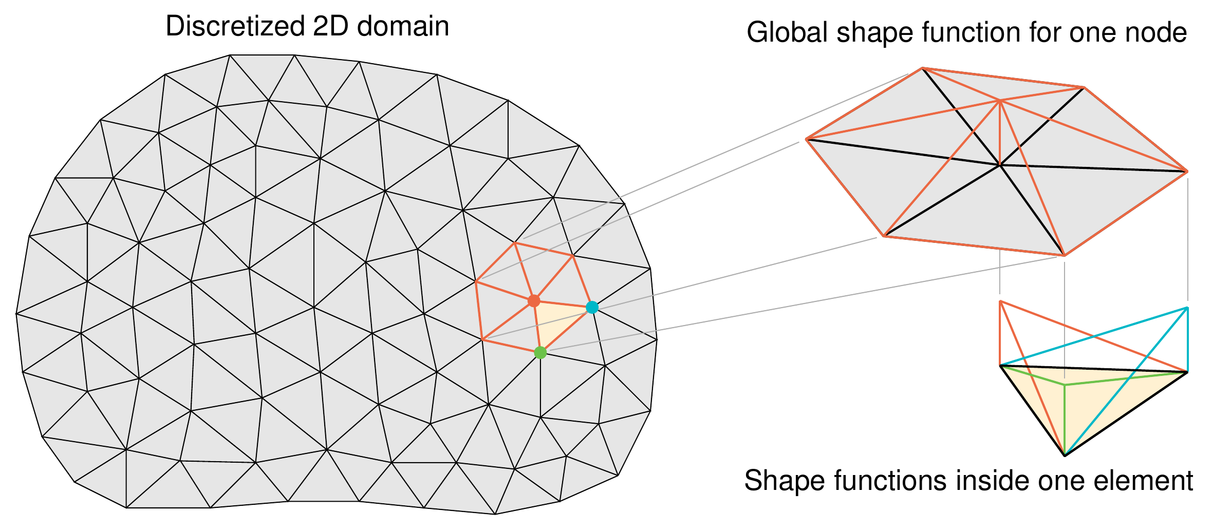
• Step 2: Discretization with Basis Functions

  The surface u is approximated as a sum of discrete nodal heights u_j(t) weighted by "tent-shaped" linear basis functions \phi_j(x,y) :

  u(x,y,t) \approx \sum_{j=1}^{N} u_j(t) \phi_j(x,y)

  • Visualization of "tent-shaped" linear basis:

    

  We test the equation against each basis function individually by setting v = \phi_i . The single integral expands into a system of equations where each corresponds to a specific node.

  \int_{\Omega} \phi_i \left( \sum_{j=1}^{N} \ddot{u}_j \phi_j \right) d\Omega + c^2 \int_{\Omega} \nabla \phi_i \cdot \left( \sum_{j=1}^{N} u_j \nabla \phi_j \right) d\Omega = 0

  This substitution separates the time-dependent nodal values from the spatial integrals.

• Step 3: Matrix Assembly (Spatial Discretization)

  The nodal values u_j and accelerations \ddot{u}_j depend only on time, while the basis functions \phi depend on spatial coordinates. Pulling the time-dependent terms out of the integrals defines the Mass ( M ) and Stiffness ( K ) matrices.

  \sum_{j=1}^{N} \ddot{u}_j \underbrace{\int_{\Omega} \phi_i \phi_j \, d\Omega}_{M_{ij}} + c^2 \sum_{j=1}^{N} u_j \underbrace{\int_{\Omega} \nabla \phi_i \cdot \nabla \phi_j \, d\Omega}_{K_{ij}} = 0

  This yields the matrix-vector equation used for the simulation:

  [M] \mathbf{\ddot{u}} + c^2 [K] \mathbf{u} = 0 \implies \mathbf{\ddot{u}} = - M^{-1}(c^2 K \mathbf{u})

  The matrices M and K are directly derived from the geometry of the triangular mesh:

  • M (Mass Matrix) : Represents the inertial weight of the water at each mesh point. It comes from the overlap of basis functions:

    M_{ij} = \int_{\Omega} \phi_i \phi_j \, d\Omega

    In the code, calculate this using the Triangle Area (lumped to the diagonal) via M_lumped .

  • K (Stiffness Matrix) : Represents the elasticity or "force" restoring the water to flat. It comes from the interaction of the slopes (gradients):

    K_{ij} = \int_{\Omega} \nabla \phi_i \cdot \nabla \phi_j \, d\Omega

    In the code, this is calculated via the gradients b and c_val , assembled as K[indices[i], indices[j]] += Ke[i, j] .

    Deriving Computation of K

    Since elements are flat triangles, the slope (gradient) of \phi is constant everywhere inside the triangle.

    K_{ij} = \int_{\triangle} (\nabla \phi_i \cdot \nabla \phi_j) \, dA

    We calculate these slopes using the geometry of the vertices:

    \nabla \phi_i = \dfrac{1}{2 \cdot \text{Area}} \begin{bmatrix} b_i \\ c_i \end{bmatrix}

    Here, b_i and c_i correspond to the geometry differences along the edges (cyclic permutations):

    • b (Slope related to y): b_0 = y_1 - y_2 , b_1 = y_2 - y_0 , b_2 = y_0 - y_1

    • c (Slope related to x): c_0 = x_2 - x_1 , c_1 = x_0 - x_2 , c_2 = x_1 - x_0

    • In the code, b and c_val store exactly these differences.

    Because the gradients are constant, the integral becomes simple multiplication (Area \times Gradient i \times Gradient j ):

    K_{ij} = \text{Area} \times \left( \dfrac{1}{2\text{Area}} \begin{bmatrix} b_i \\ c_i \end{bmatrix} \cdot \dfrac{1}{2\text{Area}} \begin{bmatrix} b_j \\ c_j \end{bmatrix} \right)

    Simplifying this yields the exact formula used in the code: Ke = (1.0 / (4.0 * Area)) * (np.outer(b, b) + np.outer(c_val, c_val))

    K_{ij} = \frac{1}{4 \cdot \text{Area}} (b_i b_j + c_i c_j)

• Step 4: Mass Lumping (Optimization)

  Standard FEM produces a coupled, sparse mass matrix ( M ), which traditionally requires a linear solver at each step. In this case, mass lumping is used for simplicity. Mass lumping approximates the inertial distribution, transforming M into a diagonal matrix, which allows for a trivial 'element-wise' inversion.

  • Benefit : M becomes a simple diagonal vector. Inverting the mass matrix is reduced to simple division, drastically speeding up the simulation.
  Deriving Computation of M

  Instead of calculating the exact overlap integral, the total area of the triangle is distributed equally to its three corners:

  M_{ii} \approx \dfrac{\text{Total Area}}{3}

  In the code, me_val = Area / 3.0 is calculated for each element and added to each vertex in the M_lumped diagonal.

• Step 5: Time Discretization (The "Loop") To step forward in time, the acceleration ( \ddot{u} ) is approximated using the Central Difference method:

  \ddot{u} \approx \frac{u^{n+1} - 2u^n + u^{n-1}}{\Delta t^2}

  Substituting this back into the global matrix equation leads to the explicit update formula used in the Python loop:

  u^{n+1} = \underbrace{2u^n - u^{n-1}}_{\text{Inertia}} - \underbrace{\Delta t^2 M^{-1} (c^2 K u^n)}_{\text{Acceleration due to Stiffness}}

  • Physics: Water accelerates in the direction that smooths out surface curvature.
  • Implementation:
    • force = K.dot(u_curr) calculates the restoring force K u^n .
    • acceleration = -force / M_lumped calculates the nodal acceleration -M^{-1} (c^2 K \mathbf{u}) .

Python Implementation and Result

The following script executes the matrix assembly and iterative update loop to produce the 2D wave visualization.

• Code Snippet

  import numpy as np
  import matplotlib.pyplot as plt
  from matplotlib.animation import FuncAnimation, PillowWriter
  from scipy.spatial import Delaunay
  from scipy.sparse import lil_matrix
  
  
  # --- 1. Configuration & Physics Setup ---
  L = 2.0  # Width of the square domain
  N = 40  # Mesh resolution (points per side)
  c = 1.0  # Wave speed
  t_final = 4.0  # Total simulation time
  fps = 20  # Animation framerate
  
  # Derived Physics Parameters
  x = np.linspace(-L / 2, L / 2, N)
  y = np.linspace(-L / 2, L / 2, N)
  X, Y = np.meshgrid(x, y)
  points = np.vstack([X.ravel(), Y.ravel()]).T
  
  # Triangulation
  tri = Delaunay(points)
  simplices = tri.simplices
  n_points = points.shape[0]
  
  # Stability (CFL Condition)
  dx_approx = L / (N - 1)
  dt = 0.5 * dx_approx / c
  
  # Animation Stepping Logic
  steps_per_frame = int(1 / (fps * dt))
  frames = int(t_final / (steps_per_frame * dt))
  
  # --- 2. FEM Matrix Assembly ---
  K = lil_matrix((n_points, n_points))
  M_lumped = np.zeros(n_points)
  
  for indices in simplices:
      pts = points[indices]
  
      # Triangle Area
      x_p, y_p = pts[:, 0], pts[:, 1]
      Area = 0.5 * np.abs(
          x_p[0] * (y_p[1] - y_p[2])
          + x_p[1] * (y_p[2] - y_p[0])
          + x_p[2] * (y_p[0] - y_p[1])
      )
  
      # Stiffness Matrix (Gradients)
      b = np.array([y_p[1] - y_p[2], y_p[2] - y_p[0], y_p[0] - y_p[1]])
      c_val = np.array([x_p[2] - x_p[1], x_p[0] - x_p[2], x_p[1] - x_p[0]])
      Ke = (1.0 / (4.0 * Area)) * (np.outer(b, b) + np.outer(c_val, c_val))
  
      # Mass Lumping
      me_val = Area / 3.0
      for i in range(3):
          M_lumped[indices[i]] += me_val
          for j in range(3):
              K[indices[i], indices[j]] += Ke[i, j]
  
  K = K.tocsr()
  
  # --- 3. Run Simulation ---
  print("Running FEM Simulation...")
  
  u_curr = np.zeros(n_points)
  u_prev = np.zeros(n_points)
  
  # Initial Condition: Pulse
  for i in range(n_points):
      dist_sq = (points[i, 0] - 0.5) ** 2 + (points[i, 1] - 0.5) ** 2
      u_curr[i] = 1.0 * np.exp(-dist_sq / 0.05)
      u_prev[i] = u_curr[i]
  
  boundary_indices = np.where(
      (np.abs(points[:, 0]) >= (L / 2 - 0.01)) | (np.abs(points[:, 1]) >= (L / 2 - 0.01))
  )[0]
  
  history = [u_curr.copy()]
  
  for frame in range(frames):
      for _ in range(steps_per_frame):
          force = K.dot(u_curr)
          acceleration = -force / M_lumped
          u_next = 2 * u_curr - u_prev + (dt**2) * acceleration
          u_next[boundary_indices] = 0
          u_prev = u_curr[:]
          u_curr = u_next[:]
      history.append(u_curr.copy())
  
  print("Simulation Complete.")
  
  # --- 4. Visualization ---
  fig = plt.figure(figsize=(6, 6))
  fig.subplots_adjust(left=0, right=1, bottom=0, top=1)
  
  ax = fig.add_subplot(111, projection="3d")
  ax.set_zlim(-1, 1)
  ax.axis("off")
  
  title_text = "2D Wave Equation (FEM)"
  time_template = "Time (t) : {:.3f}s"
  
  
  def update(frame):
      ax.clear()
      ax.set_zlim(-1, 1)
      ax.axis("off")
      ax.dist = 8
  
      u_state = history[frame]
      current_time = frame * steps_per_frame * dt
  
      ax.set_title(title_text, y=0.95)
      ax.text2D(
          0.5,
          0.85,
          time_template.format(current_time),
          transform=ax.transAxes,
          ha="center",
          va="top",
      )
  
      trisurf = ax.plot_trisurf(
          points[:, 0],
          points[:, 1],
          u_state,
          triangles=simplices,
          cmap="viridis",
          linewidth=0,
          antialiased=False,
      )
      return (trisurf,)
  
  
  ani = FuncAnimation(fig, update, frames=len(history), interval=1000 / fps)
  
  # --- 5. Save GIF ---
  print("Saving GIF...")
  writer = PillowWriter(fps=fps)
  ani.save("wave_fem.gif", writer=writer)
  print("Saved to wave_fem.gif")
  

• Result

  

Case 2: Obstacle Hole

Physical Environment:

• Domain: \Omega = [-1, 1] \times [-1, 1] \setminus \mathcal{O} , representing a square pool with a circular hole of radius r=0.5 centered at the origin.

• Initial Condition : Flat water surface ( u=0 ) with a Gaussian droplet peak located at [0.8, 0.8] .

• Boundary Conditions:
  • Outer Boundary ( \partial \Omega_{ext} ): Homogeneous Dirichlet ( u=0 ), fixing the water height at the walls.
  • Obstacle Boundary ( \partial \Omega_{int} ): Homogeneous Neumann ( \nabla u \cdot \mathbf{n} = 0 ), where \mathbf{n} is the normal vector to the circle.
  • Physics : The Neumann condition ensures the wave's slope is zero at the boundary, forcing it to 'bounce' back without losing energy.

• Mesh : Unstructured triangular mesh that conforms exactly to the circular boundary of the obstacle.

Unstable Implementation and Result

Updating the configuration with a circular hole triggers a numerical blow-up. High-frequency oscillations grow into the divergent spikes shown below, necessitating the stability analysis in the next section.

• Code Snippet

  import numpy as np
  import matplotlib.pyplot as plt
  from matplotlib.animation import FuncAnimation, PillowWriter
  from scipy.spatial import Delaunay
  from scipy.sparse import lil_matrix
  
  
  # --- 1. Configuration & Physics Setup ---
  L = 2.0  # Width of the square domain
  N = 50  # Mesh resolution (points per side)
  c = 1.5  # Wave speed
  t_final = 4.0  # Total simulation time
  fps = 20  # Animation framerate
  hole_radius = 0.5
  
  # Derived Physics Parameters
  x = np.linspace(-L / 2, L / 2, N)
  y = np.linspace(-L / 2, L / 2, N)
  X, Y = np.meshgrid(x, y)
  points = np.vstack([X.ravel(), Y.ravel()]).T
  
  # Remove points inside the hole
  dist = np.linalg.norm(points, axis=1)
  points = points[dist > hole_radius]
  
  # Triangulation
  tri = Delaunay(points)
  simplices = tri.simplices
  
  # Remove triangles inside the hole
  centroids = np.mean(points[simplices], axis=1)
  simplices = simplices[np.linalg.norm(centroids, axis=1) > hole_radius]
  
  n_points = points.shape[0]
  
  # Stability (CFL Condition) - THE SOURCE OF INSTABILITY
  # We estimate dx based on average spacing, ignoring tiny cut elements
  dx_approx = L / (N - 1)
  dt = 0.5 * dx_approx / c
  
  # Animation Stepping Logic
  steps_per_frame = int(1 / (fps * dt))
  frames = int(t_final / (steps_per_frame * dt))
  
  # --- 2. FEM Matrix Assembly ---
  K = lil_matrix((n_points, n_points))
  M_lumped = np.zeros(n_points)
  
  for indices in simplices:
      pts = points[indices]
  
      # Triangle Area
      x_p, y_p = pts[:, 0], pts[:, 1]
      Area = 0.5 * np.abs(
          x_p[0] * (y_p[1] - y_p[2])
          + x_p[1] * (y_p[2] - y_p[0])
          + x_p[2] * (y_p[0] - y_p[1])
      )
  
      # Stiffness Matrix (Gradients)
      b = np.array([y_p[1] - y_p[2], y_p[2] - y_p[0], y_p[0] - y_p[1]])
      c_val = np.array([x_p[2] - x_p[1], x_p[0] - x_p[2], x_p[1] - x_p[0]])
      Ke = (1.0 / (4.0 * Area)) * (np.outer(b, b) + np.outer(c_val, c_val))
  
      # Mass Lumping
      me_val = Area / 3.0
      for i in range(3):
          M_lumped[indices[i]] += me_val
          for j in range(3):
              K[indices[i], indices[j]] += Ke[i, j]
  
  K = K.tocsr()
  
  # --- 3. Run Simulation ---
  print("Running FEM Simulation...")
  
  u_curr = np.zeros(n_points)
  u_prev = np.zeros(n_points)
  
  # Initial Condition: Pulse
  for i in range(n_points):
      dist_sq = (points[i, 0] - 0.8) ** 2 + (points[i, 1] - 0.8) ** 2
      u_curr[i] = 1.0 * np.exp(-dist_sq / 0.05)
      u_prev[i] = u_curr[i]
  
  boundary_indices = np.where(
      (np.abs(points[:, 0]) >= (L / 2 - 0.01)) | (np.abs(points[:, 1]) >= (L / 2 - 0.01))
  )[0]
  
  history = [u_curr.copy()]
  
  for frame in range(frames):
      for _ in range(steps_per_frame):
          force = K.dot(u_curr)
          acceleration = -force / M_lumped
          u_next = 2 * u_curr - u_prev + (dt**2) * acceleration
          u_next[boundary_indices] = 0
          u_prev = u_curr[:]
          u_curr = u_next[:]
      history.append(u_curr.copy())
  
  print("Simulation Complete.")
  
  # --- 4. Visualization ---
  fig = plt.figure(figsize=(6, 6))
  fig.subplots_adjust(left=0, right=1, bottom=0, top=1)
  
  ax = fig.add_subplot(111, projection="3d")
  ax.set_zlim(-1, 1)
  ax.axis("off")
  
  title_text = "2D Wave Equation (FEM) with Hole"
  time_template = "Time (t) : {:.3f}s"
  
  r_hole = np.linspace(0, hole_radius, 20)
  theta_hole = np.linspace(0, 2 * np.pi, 50)
  R_hole, Theta_hole = np.meshgrid(r_hole, theta_hole)
  X_hole = R_hole * np.cos(Theta_hole)
  Y_hole = R_hole * np.sin(Theta_hole)
  Z_hole = np.zeros_like(X_hole)  # Flat at z=0
  
  
  def update(frame):
      ax.clear()
      ax.set_zlim(-1, 1)
      ax.axis("off")
      ax.dist = 8
  
      u_state = history[frame]
      current_time = frame * steps_per_frame * dt
  
      ax.set_title(title_text, y=0.95)
      ax.text2D(
          0.5,
          0.85,
          time_template.format(current_time),
          transform=ax.transAxes,
          ha="center",
          va="top",
      )
  
      ax.plot_trisurf(
          points[:, 0],
          points[:, 1],
          u_state,
          triangles=simplices,
          cmap="viridis",
          linewidth=0,
          antialiased=False,
      )
      ax.plot_surface(X_hole, Y_hole, Z_hole, color="black", alpha=1.0, shade=False)
  
      return (ax,)
  
  
  ani = FuncAnimation(fig, update, frames=len(history), interval=1000 / fps)
  
  # --- 5. Save GIF ---
  print("Saving GIF...")
  writer = PillowWriter(fps=fps)
  ani.save("wave_fem_hole_unstable.gif", writer=writer)
  print("Saved to wave_fem_hole_unstable.gif")
  

• Result

  

Case 2.5: Geometry and Stability Analysis

Why the previous code was unstable?

The instability was caused by a Courant-Friedrichs-Lewy (CFL) violation.

The Geometry Problem (Sliver Triangles)

When points inside the circle are deleted from a square grid, the remaining points near the boundary form a jagged edge.

The Delaunay triangulator connects these jagged points, creating needle-like triangles called slivers. These triangles have a near-zero altitude ( h \approx 0 ).

The Math Problem (CFL Condition)

Stability in explicit solvers is governed by the CFL condition, which mandates that the numerical 'domain of dependence' must encompass the physical 'domain of dependence.'

In practice, \Delta t must be small enough that the wave does not leapfrog across an entire element in a single step:

The unstable code estimated \Delta t using average grid spacing ( h \approx 0.04 ). However, the actual h_{\text{min}} due to slivers was approximately 0.0001 . Since the calculated \Delta t was much larger than the slivers could handle, the simulation blew up at the hole boundary.

Approaches for Robust Solution

1. Boundary Conforming Meshing : Explicitly generating ring points around the hole forces the Delaunay triangulation to respect the circular boundary. This replaces jagged slivers with a clean fan shape.

2. CFL-Aware Time Stepping : Calculating the height h for every triangle during assembly identifies the true global minimum h_{\text{min}} . Setting \Delta t based on this minimum guarantees stability for every element.

Robust Implementation and Result

By implementing boundary conforming points and a CFL-aware time step, the simulation achieves stability. The waves reflect naturally off the circular obstacle without numerical divergence.

• Code Snippet

  import numpy as np
  import matplotlib.pyplot as plt
  from matplotlib.animation import FuncAnimation, PillowWriter
  from scipy.spatial import Delaunay
  from scipy.sparse import lil_matrix
  
  
  # --- 1. Configuration & Physics Setup ---
  L = 2.0  # Width of the square domain
  N = 50  # Mesh resolution (points per side)
  c = 1.5  # Wave speed
  t_final = 4.0  # Total simulation time
  fps = 20  # Animation framerate
  hole_radius = 0.5
  
  # --- 2. Robust Mesh Generation ---
  x = np.linspace(-L / 2, L / 2, N)
  y = np.linspace(-L / 2, L / 2, N)
  X, Y = np.meshgrid(x, y)
  points = np.vstack([X.ravel(), Y.ravel()]).T
  
  # Remove points inside the hole strictly (with a small buffer)
  dist = np.linalg.norm(points, axis=1)
  points = points[dist > hole_radius + 0.02]
  
  # Explicitly add points on the hole boundary to ensure shape conformity
  # This prevents "jagged" edges and sliver triangles
  theta = np.linspace(0, 2 * np.pi, 100)
  ring_points = np.vstack([hole_radius * np.cos(theta), hole_radius * np.sin(theta)]).T
  points = np.vstack([points, ring_points])
  
  # Triangulation & Filtering
  tri = Delaunay(points)
  simplices = tri.simplices
  
  # Remove triangles inside the hole
  centroids = np.mean(points[simplices], axis=1)
  simplices = simplices[np.linalg.norm(centroids, axis=1) > hole_radius + 1e-4]
  
  # Topology Cleaning (Remove unused points)
  unique_indices = np.unique(simplices)
  idx_map = {old: new for new, old in enumerate(unique_indices)}
  points = points[unique_indices]
  simplices = np.vectorize(idx_map.get)(simplices)
  n_points = points.shape[0]
  
  # --- 3. FEM Matrix Assembly & Stability Check ---
  K = lil_matrix((n_points, n_points))
  M_lumped = np.zeros(n_points)
  min_h = 1.0  # Track minimum element size
  
  for indices in simplices:
      pts = points[indices]
  
      # Triangle Area
      x_p, y_p = pts[:, 0], pts[:, 1]
      Area = 0.5 * np.abs(
          x_p[0] * (y_p[1] - y_p[2])
          + x_p[1] * (y_p[2] - y_p[0])
          + x_p[2] * (y_p[0] - y_p[1])
      )
      if Area < 1e-12:
          continue
  
      # STABILITY FIX: Calculate Characteristic Length (h)
      # h = 2 * Area / max_edge_length (Altitude approximation)
      edge_lens = [
          np.sqrt((x_p[i] - x_p[j]) ** 2 + (y_p[i] - y_p[j]) ** 2)
          for i, j in [(0, 1), (1, 2), (2, 0)]
      ]
      h = 2.0 * Area / np.max(edge_lens)
      min_h = min(min_h, h)
  
      # Stiffness Matrix (Gradients)
      b = np.array([y_p[1] - y_p[2], y_p[2] - y_p[0], y_p[0] - y_p[1]])
      c_val = np.array([x_p[2] - x_p[1], x_p[0] - x_p[2], x_p[1] - x_p[0]])
      Ke = (1.0 / (4.0 * Area)) * (np.outer(b, b) + np.outer(c_val, c_val))
  
      # Mass Lumping
      me_val = Area / 3.0
      for i in range(3):
          M_lumped[indices[i]] += me_val
          for j in range(3):
              K[indices[i], indices[j]] += Ke[i, j]
  
  K = K.tocsr()
  
  # --- 4. Adaptive Time Step Calculation ---
  # CFL Condition: dt <= C * h_min / c
  # We use the ACTUAL minimum height found in the mesh, not an average guess.
  dt = 0.6 * min_h / c
  print(f"Computed Stable dt: {dt:.6e} s (min_h: {min_h:.6e})")
  
  # Animation Stepping Logic
  steps_per_frame = int(1 / (fps * dt))
  frames = int(t_final / (steps_per_frame * dt))
  
  # --- 5. Run Simulation ---
  print("Running FEM Simulation...")
  
  u_curr = np.zeros(n_points)
  u_prev = np.zeros(n_points)
  
  # Initial Condition: Pulse
  for i in range(n_points):
      dist_sq = (points[i, 0] - 0.8) ** 2 + (points[i, 1] - 0.8) ** 2
      u_curr[i] = 1.0 * np.exp(-dist_sq / 0.05)
      u_prev[i] = u_curr[i]
  
  boundary_indices = np.where(
      (np.abs(points[:, 0]) >= (L / 2 - 0.01)) | (np.abs(points[:, 1]) >= (L / 2 - 0.01))
  )[0]
  
  history = [u_curr.copy()]
  
  for frame in range(frames):
      for _ in range(steps_per_frame):
          force = K.dot(u_curr)
          acceleration = -force / M_lumped
          u_next = 2 * u_curr - u_prev + (dt**2) * acceleration
          u_next[boundary_indices] = 0
          u_prev = u_curr[:]
          u_curr = u_next[:]
      history.append(u_curr.copy())
  
  print("Simulation Complete.")
  
  # --- 6. Visualization ---
  fig = plt.figure(figsize=(6, 6))
  fig.subplots_adjust(left=0, right=1, bottom=0, top=1)
  
  ax = fig.add_subplot(111, projection="3d")
  ax.set_zlim(-1, 1)
  ax.axis("off")
  
  title_text = "2D Wave Equation (FEM) with Hole"
  time_template = "Time (t) : {:.3f}s"
  
  r_hole = np.linspace(0, hole_radius, 20)
  theta_hole = np.linspace(0, 2 * np.pi, 50)
  R_hole, Theta_hole = np.meshgrid(r_hole, theta_hole)
  X_hole = R_hole * np.cos(Theta_hole)
  Y_hole = R_hole * np.sin(Theta_hole)
  Z_hole = np.zeros_like(X_hole)  # Flat at z=0
  
  
  def update(frame):
      ax.clear()
      ax.set_zlim(-1, 1)
      ax.axis("off")
      ax.dist = 8
  
      u_state = history[frame]
      current_time = frame * steps_per_frame * dt
  
      ax.set_title(title_text, y=0.95)
      ax.text2D(
          0.5,
          0.85,
          time_template.format(current_time),
          transform=ax.transAxes,
          ha="center",
          va="top",
      )
  
      ax.plot_trisurf(
          points[:, 0],
          points[:, 1],
          u_state,
          triangles=simplices,
          cmap="viridis",
          linewidth=0,
          antialiased=False,
      )
      ax.plot_surface(X_hole, Y_hole, Z_hole, color="black", alpha=1.0, shade=False)
  
      return (ax,)
  
  
  ani = FuncAnimation(fig, update, frames=len(history), interval=1000 / fps)
  
  # --- 7. Save GIF ---
  print("Saving GIF...")
  writer = PillowWriter(fps=fps)
  ani.save("wave_fem_hole_robust.gif", writer=writer)
  print("Saved to wave_fem_hole_robust.gif")
  

• Result