Everyone doing deep learning (DL) knows Adam. It has been the default in every framework, rarely questioned. Over the past year it stopped being the default at the labs training the largest models.
Muon
is what Moonshot used for Moonlight
[2] and then Kimi K2 at 1T parameters
[1], and what Z.ai used for GLM-4.5
[3].
Why not Adam?
Adam is not broken. It stops being the right tool at scale, for two reasons with a common root: it treats a weight matrix as a bag of independent numbers.
Problem 1: the update is measured in the wrong unit
"Width" here means the hidden dimension, and it is the axis that has moved most. The original Transformer used 512, BERT-large 1024. Kimi K2 uses 7168.
An effect you could ignore at 512 decides the run at 7168.
As width grows, a model trained under standard parameterization barely leaves where it started. The same freeze appears, for a different scaling, in the infinite-width NTK parametrization
[4]:
In the infinite-width limit, training is governed by a kernel that is fixed at initialization and stays constant throughout.
Yang and Hu made the statement sharp: the standard and NTK parameterizations admit no infinite-width limit that learns features
[6]. This is not slow convergence that more steps would cure. The limit itself cannot learn features.
Maximal update parametrization (µP) is the repair
[6].
It rescales per-layer learning rates and initializations so that representations evolve at every width.
Hyperparameters tuned on a small model then transfer to a large one
[7].
µP deserves its own post and will get one. Here it is enough to know what it fixes.
So what is the quantity that has to be held fixed? The spectral condition answers it directly
[8]. A hidden weight
W\in\mathbb{R}^{m\times n}
maps
n
incoming activations to
m
outgoing ones:
n
is the
fan-in,
m
the
fan-out. For a square layer they are the same number, and that number is the width.
"feature learning is achieved by scaling the spectral norm of weight matrices and their updates like √(fan-out/fan-in), in contrast to widely used but heuristic scalings based on
Frobenius norm and entry size."
The last clause names two heuristics, and the paper stops there. The daily optimizers under those heuristics are easy to name: Frobenius norm is the ruler of normalized SGD. Entry size is the ruler of Adam.
Adam's update is
m/\sqrt{v}:
m
a running mean of the gradient,
v
of its square. Turn the averaging off and they collapse to the current gradient and its square,
m = g
and
v = g^2
elementwise, so the update is
Each entry is decided on its own
[11]. What it holds constant is the size of that entry, whatever the shape of the matrix. That is the wrong invariant, and
the error grows with width.
💡
Adam's step is not too large or too small. It is measured with the wrong ruler.
Problem 2: the update points in too few directions
The second failure is visible without any theory. Updates produced by SGD-momentum and by Adam on a transformer's 2D parameters have very high condition number
[9].
They are close to low-rank:
a handful of singular directions carry almost the entire step, and the rest of the neurons receive nearly nothing.
That is waste. Whatever signal the remaining directions carried is thrown away, every step, and the wider the layer the more of them there are to throw away.
Two failures, then. One about how the step is measured, one about where it points. Neither is a bug in Adam's implementation. Both follow from never looking at the matrix as a map.
Why Muon?
Here is the whole method in one sentence:
💡
Take the momentum, orthogonalize it with a few Newton–Schulz iterations, and use that as the update.
That sentence has two halves, and each one answers one of the two problems.
Orthogonalization answers Problem 2
Replace the momentum by the nearest matrix whose singular values are all 1.
The directions already present are preserved, their magnitudes are discarded, and every one of them receives a step of the same size.
The low-rank update is not damped or regularized. Every singular value that carried any signal is set to 1, so a handful of directions can no longer take the whole step.
Scaling answers Problem 1
Orthogonalization sets every singular value of
UV^T
to
1, so the largest one (the spectral norm) is
1
at any shape.
Adam never looks at it. Adam rescales entries, and the singular values stay as peaked as they were
[9].
That does not freeze a typical entry. The sum of squares of the entries equals the sum of squares of the singular values. Write that sum as
\|A\|_F^2.
After orthogonalization those singular values are all
1. If the momentum is full rank there are
\min(m,n)
of them, so for
W\in\mathbb{R}^{m\times n}
\|UV^T\|_F^2 = \min(m,n)
Write
\mathrm{RMS}
for the root-mean-square of the entries, the square root of the average squared entry:
Adam's update entries stay
O(1)
at any width.
\mathrm{RMS}(UV^T)
does not.
A multiplier that depends on
m
and
n
still has to be chosen, or the same
\eta
makes the Muon step shrink next to AdamW.
Moonlight and the usual implementation multiply by
0.2\sqrt{\max(m,n)}. The scaled polar factor then has entry RMS near
0.2, so
\Delta W
has entry RMS near
0.2\eta
and the two groups can share a learning rate
[2].
Adam
Muon
what it holds constant
size of a single entry
\sigma_{\max}(UV^T)=1
at any shape
where the step points
the peaked spectrum of
G
every direction already present
Setting every singular value to 1 is a strange operation to arrive at by intuition, and there are other ways to make an update less low-rank. The next section asks what steepest descent means once the step is measured as a matrix. The answer is
UV^T.
Where Orthogonalization Comes From
This section follows Bernstein’s derivation
[10]. The idea that each optimizer is steepest descent under some norm is from his work with Newhouse
[11]. Similar ideas appeared earlier in stochastic spectral descent
[12]
and duality structure gradient descent
[13].
Optimizers choose a geometry
Given an objective
f, everyone already knows gradient descent:
\theta \leftarrow \theta - \eta \nabla_{\theta} f. It feels like the natural move. The geometry that produces it is easy to miss.
Start from basic calculus on
f:\mathbb{R}^n\to\mathbb{R}.
At a point, the directional derivative
D_v f
may exist even if one does not want to talk about a gradient. The gradient is defined by
\langle \nabla f, v \rangle = D_v f
for every direction
v.
Taylor expansion writes the same pairing as a predicted change in the loss:
So\nabla_{\theta} fis not a list of partials sitting in a vacuum. It requires a pairing\langle,\rangle.
The pairing is the component that determines the geometry:
\langle,\rangle = \langle,\rangle_g, so we write the subscript as well.
On Euclidean space,
\langle,\rangle_g
is the ordinary dot product.
In another geometry,
\langle v, w\rangle_g
can be
v^T M w
for some positive-definite matrix
M.
For matrices that pairing is the Frobenius product
\mathrm{tr}(v^T w). It does not pick the optimizer.
The ball does.
Trust the linear model only near
\theta
and bound the step:
The objective never changes. Only the ball does, and that is enough to change the answer. The inner problem is the
linear minimization oracle (LMO)
of that ball. The
v
that attains it is the update direction.
The Euclidean ball gives normalized SGD.
With the Frobenius norm
\|v\|_F, Cauchy–Schwarz gives
\langle \nabla_{\theta} f, v\rangle \le \|\nabla_{\theta} f\|_F, with equality when
v
points along
\nabla_{\theta} f:
\mathrm{LMO}_F(\nabla_{\theta} f) = \nabla_{\theta} f / \|\nabla_{\theta} f\|_F.
This is the only sense in which "
-\nabla f
is the steepest direction" is true, and it is true only if a step’s size is the sum of squares of its entries.
Vanilla SGD takes that direction and skips the projection onto the unit ball.
The entrywise ball gives signSGD.
With
\|v\|_\infty = \max_{ij}|v_{ij}|, a step is allowed as long as no entry exceeds 1 in absolute value.
The pairing splits across entries,
\langle \nabla_{\theta} f, v\rangle = \sum_{ij}(\nabla_{\theta} f)_{ij} v_{ij}, and each term is maximized by
v_{ij}=\mathrm{sign}((\nabla_{\theta} f)_{ij}). So
\mathrm{LMO}_\infty(\nabla_{\theta} f)=\mathrm{sign}(\nabla_{\theta} f).
In this geometry a step’s size is its largest entry. "
-\nabla f
is the steepest direction" is simply false here.
Adam is
m/\sqrt{v}. EMA off and that is
\mathrm{sign}(\nabla_{\theta} f)
[11], the same entrywise ruler as Problem 1.
Norm on
\Delta
\mathrm{LMO}(\nabla_{\theta} f)
Optimizer
Frobenius
\nabla_{\theta} f/\|\nabla_{\theta} f\|_F
normalized SGD
entrywise max
\mathrm{sign}(\nabla_{\theta} f)
signSGD; Adam with EMAs off
spectral
?
?
The third row is the one we want. What remains is to compute it.
The spectral ball gives
UV^T
Both norms above treat
W \in \mathbb{R}^{m \times n}
as
mn
unrelated scalars. Shuffle the entries and neither notices. A hidden weight is the map
h = Wx. A step
\Delta
on
W, with
x
held fixed, moves the output by
\Delta x:
(W+\Delta)x = h + \Delta x
The rest of the model receives
\Delta x.
So the size of
\Delta
is the largest output displacement it can cause, relative to the
x
that produced it. Measure activations in RMS: typical entry size is what we care about, and widths differ. The induced operator norm is
where
\sigma_{\max}is the spectral norm, the largest singular value. The factor in front is set by the layer’s shape.
Now bound the update in that norm.
\|\Delta\|_{\mathrm{RMS}\to\mathrm{RMS}} \le \eta
is the same as
\sigma_{\max}(\Delta) \le \eta\sqrt{\texttt{fan-out}/\texttt{fan-in}}, so the problem is an LMO over a spectral ball:
\argmax_{\sigma_{\max}(v) \le 1} \langle \nabla_{\theta} f, v \rangle = UV^T
where
\nabla_{\theta} f = U\Sigma V^T
is the reduced SVD.
Proof
Write the objective as a Frobenius inner product and rotate:
The constraint does not care about an orthogonal change of basis, so
M := U^T \Delta V
still has
\sigma_{\max}(M) \le 1, hence
|M_{ii}| \le 1. Every
\sigma_i \ge 0, so
with equality when
M = I_r, i.e.
\Delta = UV^T, the polar factor of
\nabla_{\theta} f.
If the matrix is rectangular, this identity lives only on the reduced
r
-dimensional factors:
UV^T
has orthonormal rows or orthonormal columns, not both.
UV^T
is the polar factor of
\nabla_{\theta} f: the nearest semi-orthogonal matrix in Frobenius
[9]. For full-rank momentum that is the same as setting every singular value to 1.
That is Muon,
MomentUm
Orthogonalized by
Newton-Schulz: the momentum buffer stands in for
\nabla_{\theta} f, and Newton–Schulz is how
UV^T
is computed.
Restoring the shape factor gives Bernstein’s update:
\Delta W = -\eta\sqrt{\dfrac{\texttt{fan-out}}{\texttt{fan-in}}}\,UV^T
The implementation and Moonlight keep
UV^T
and replace the prefactor
[2]:
\Delta W = -\eta\cdot 0.2\sqrt{\max(m,n)}\,UV^T
Bernstein holds
\|\Delta W\|_{\mathrm{RMS}\to\mathrm{RMS}}=\eta: how far the layer can move its output.
Moonlight holds the entry RMS of
\Delta W
at
0.2\eta, so a Muon group and an AdamW group can share a learning rate.
On a square layer the two prefactors are
1
and
0.2\sqrt{n}. Bernstein expects his factor to scale better
[10].
They do not disagree on a constant. They disagree on which size is being held fixed.
This also explains Problem 2 rather than merely fixing it. The Frobenius ball prices a step by total squared magnitude and is indifferent to how that magnitude is spread across directions, so the budget goes to whichever two or three directions carry the largest gradient signal.
Adam never does that mixing either: it rescales entries, and the peaked spectrum of
G
is still there
[9]. The near low-rank update was never a defect in the implementation. It is what you get when the geometry never looks at
G
as a map.
Norm on
\Delta
\mathrm{LMO}(\nabla_{\theta} f)
Optimizer
Frobenius
\nabla_{\theta} f/\|\nabla_{\theta} f\|_F
normalized SGD
entrywise max
\mathrm{sign}(\nabla_{\theta} f)
signSGD; Adam with EMAs off
spectral
UV^T
Muon
If the step is measured by how far it can move the layer's output, the constraint returns
UV^T.
Making It Actually Run
UV^T
is the update. The obvious computation is an SVD of every 2D weight at every step. That is too slow at this frequency, and bf16 will not keep
U
and
V
honest. What follows is
UV^T
with no
U
and no
V.
UV^T
from matmuls
The lemma that makes it possible
Consider an
odd
matrix polynomial built from
X
and
X^T X:
p(X) = aX + bX(X^T X) + cX(X^T X)^2
Substitute
X = U\Sigma V^T. Since
X^T X = V\Sigma^2 V^T, we get
X(X^T X)^k = U\Sigma^{2k+1}V^T, and by linearity:
The singular vectors are untouched. The polynomial acts only on the singular values, one at a time.
That is the whole trick, and it reduces a matrix problem to a scalar one:
Find an odd scalar polynomialpsuch that iterating it drives everys \in (0,1]toward1.
Do that, and
k
iterations applied to
\nabla_{\theta} f
produce
Up^{\circ k}(\Sigma)V^T \approx UV^T
using nothing but matrix multiplications, the one operation GPUs are extravagantly good at.
Let
G
be the matrix Newton–Schulz sees, the momentum. The restriction to
(0,1]
is why the implementation divides by
\|G\|_F
first.
\sigma_{\max}(G)\le\|G\|_F, so this puts every singular value in
(0,1].
The iteration does not converge, and that is deliberate
The textbook Newton–Schulz iteration for the polar factor
[17]
is the cubic
p(x)=\tfrac{3}{2}x-\tfrac{1}{2}x^3. The same family has a degree-5 member
(a,b,c)=(\tfrac{15}{8},-\tfrac{10}{8},\tfrac{3}{8}), which also converges to
1
quadratically.
Muon does not use it. It uses
(a, b, c) = (3.4445, -4.7750, 2.0315), and iterating them does not converge to anything. Read them straight off:
p(1) = 3.4445 - 4.7750 + 2.0315 = 0.701, so
s=1
is
not
a fixed point.
p(s)=s
gives
s=0
or
2.0315s^4 - 4.7750s^2 + 2.4445 = 0: nonzero roots
s \approx 0.868
and
s \approx 1.264.
Both are repelling
p'(0.868) \approx -1.58,
p'(1.264) \approx 6.47, so
|p'| > 1
at each.
On
[0,1],
p
rises to a maximum of
\approx 1.202
at
s \approx 0.554, then falls back to
0.701.
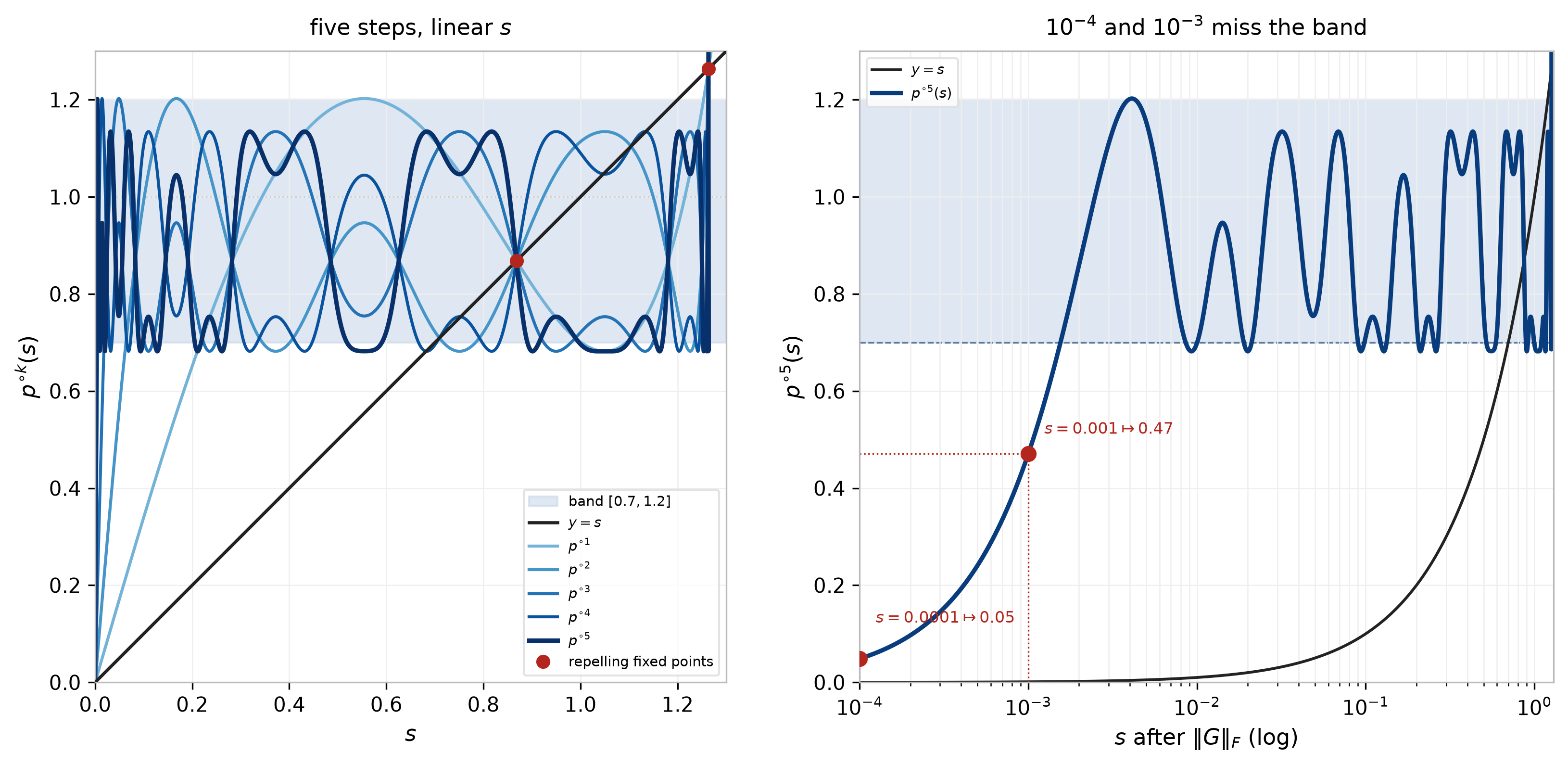
There is no stable fixed point anywhere. Singular values never converge to
1. After enough iterations they cycle in roughly
[0.68, 1.13]. The usual description is a band of
[0.7, 1.2]
[9,16].
Muon uses five steps and stops.
p'(0)=3.4445
against
15/8=1.875
for that convergent quintic, so small singular values rise faster. Jianlin Su’s guide
[14]
works through the practical consequences.
💡
Muon's Newton–Schulz is not an approximation that would be better if it were exact. It is a deliberately inexact map, tuned against a wall-clock budget of five matmul rounds.
Divide
G
by
\|G\|_F. Singular values now lie in
(0,1]. Five applications of
p
put most of them in
[0.7,1.2]. The small ones stay small:
10^{-3}
comes out
0.47,
10^{-4}
comes out
0.05. Those directions of
W
move by
0.47
and
0.05, not by
1.
Figure.
Left:
p^{\circ k}
against
y=s. Right:
p^{\circ 5}
on a log-
s
axis, with
10^{-3}
and
10^{-4}
marked.
Gram Newton–Schulz
[15]
is the same odd polynomial, rewritten so the iteration runs on the small Gram (
XX^T
after the short-side transpose; the lemma used
X^T X
). In exact arithmetic it returns the same
UV^T.
Chebyshev-type accelerations
[16]
use a different composition of odd polynomials, with a steeper slope at
0, so more of the small singular values move at a similar matmul budget.
How Do We Turn It Into a Real Optimizer?
UV^T
is one matrix. A transformer run needs three more decisions.
Which parameters.
Muon goes on hidden 2D weights. Embeddings, the LM head, and 1D parameters stay on AdamW.
An embedding table takes a one-hot index. Each row updates alone, not as one map
h=Wx. The first conv layer fails the same test: its input is pixels.
The LM head still maps a dense hidden state. Most runs still leave it on AdamW: the output is logits, fan-out is the vocabulary, and the weights are often tied to the embedding.
The multiplier.
Three formulas, PyTorch layout
(m,n)=(\texttt{fan-out},\texttt{fan-in}):
Jordan:
\sqrt{\max(1,m/n)}
[9]. Same as Bernstein when
m\ge n; not when the layer shrinks.
Moonlight:
0.2\sqrt{\max(m,n)}, entry RMS
\sim 0.2, so AdamW can share
\eta
[2].
Decoupled weight decay.\mathrm{LMO}(\alpha\nabla_{\theta} f)=\mathrm{LMO}(\nabla_{\theta} f)
for any
\alpha>0: the step does not grow or shrink with
\|\nabla_{\theta} f\|. That is not unique to Muon.
At scale the weights still drift up and the effective learning rate drifts down. Decoupled weight decay is reported as necessary once you leave the original NanoGPT setting
[2].
The whole thing, in about forty lines
import torch


def newton_schulz(G, steps=5, eps=1e-7):
    """Approximate the orthogonal polar factor UV^T of G via a quintic odd polynomial."""
    a, b, c = 3.4445, -4.7750, 2.0315
    X = G.bfloat16()
    X = X / (X.norm() + eps)  # force all singular values into (0, 1]
    transposed = G.size(0) > G.size(1)
    if transposed:  # run NS on the short side
        X = X.T

    for _ in range(steps):
        A = X @ X.T  # p(X) = aX + bAX + cA^2X
        B = b * A + c * (A @ A)
        X = a * X + B @ X

    return X.T if transposed else X


class Muon(torch.optim.Optimizer):
    def __init__(self, params, lr=2e-4, momentum=0.95, weight_decay=0.1, nesterov=True):
        # Moonlight/K2/GLM: AdamW-scale η with 0.2√max. Jordan used 0.02 with √max(1,m/n).
        super().__init__(
            params,
            dict(
                lr=lr, momentum=momentum, weight_decay=weight_decay, nesterov=nesterov
            ),
        )

    @torch.no_grad()
    def step(self):
        for group in self.param_groups:
            mu, lr, wd = group["momentum"], group["lr"], group["weight_decay"]
            for p in group["params"]:
                if p.grad is None:
                    continue
                assert p.ndim == 2, (
                    "Muon is for hidden 2D weights; flatten convs first, AdamW elsewhere"
                )
                state = self.state[p]
                if "buf" not in state:
                    state["buf"] = torch.zeros_like(p)
                buf = state["buf"]
                buf.lerp_(p.grad, 1 - mu)
                g = p.grad.lerp(buf, mu) if group["nesterov"] else buf

                u = newton_schulz(g).to(p.dtype)  # polar factor; spectral LMO
                scale = 0.2 * max(p.shape) ** 0.5  # Moonlight RMS match, not Bernstein

                p.mul_(1 - lr * wd)  # decoupled weight decay
                p.add_(u, alpha=-lr * scale)
This section makes the step run. A real optimizer still has to share a schedule with AdamW, keep a QK product bounded, and orthogonalize a matrix the cluster does not hold. That is About Muon: Muon At Scale.
[2] Liu, J., Su, J., Yao, X., et al. (2025, February). Muon is Scalable for LLM Training. arXiv:2502.16982.
https://arxiv.org/abs/2502.16982
[3] GLM-4.5 Team. (2025, August). GLM-4.5: Agentic, Reasoning, and Coding (ARC) Foundation Models. arXiv:2508.06471.
https://arxiv.org/abs/2508.06471
[4] Jacot, A., Gabriel, F., & Hongler, C. (2018, June 20). Neural Tangent Kernel: Convergence and Generalization in Neural Networks. arXiv:1806.07572.
https://arxiv.org/abs/1806.07572
[5] Chizat, L., Oyallon, E., & Bach, F. (2018, December 19). On Lazy Training in Differentiable Programming. arXiv:1812.07956.
https://arxiv.org/abs/1812.07956
[6] Yang, G., & Hu, E. J. (2020, November 30). Feature Learning in Infinite-Width Neural Networks. arXiv:2011.14522.
https://arxiv.org/abs/2011.14522
[7] Yang, G., Hu, E. J., Babuschkin, I., Sidor, S., Liu, X., Farhi, D., Ryder, N., Pachocki, J., Chen, W., & Gao, J. (2022, March 7). Tensor Programs V: Tuning Large Neural Networks via Zero-Shot Hyperparameter Transfer. arXiv:2203.03466.
https://arxiv.org/abs/2203.03466
[8] Yang, G., Simon, J. B., & Bernstein, J. (2023, October 26). A Spectral Condition for Feature Learning. arXiv:2310.17813.
https://arxiv.org/abs/2310.17813
[13] Flynn, T. (2017, August). The Duality Structure Gradient Descent Algorithm: Analysis and Applications to Neural Networks. arXiv:1708.00523.
https://arxiv.org/abs/1708.00523
[16] Grishina, E., Smirnov, M., & Rakhuba, M. (2025, June 12). Accelerating Newton-Schulz Iteration for Orthogonalization via Chebyshev-type Polynomials. arXiv:2506.10935.
https://arxiv.org/abs/2506.10935