Why EM?

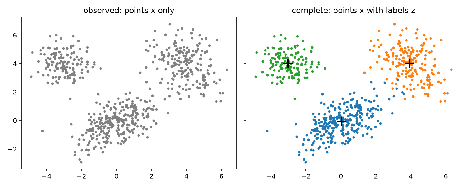
Suppose we observe the 600 points in the left panel and assume they come from three Gaussian clusters. Fitting this Gaussian mixture means estimating a weight, a mean and a covariance for each cluster.

If we knew which cluster produced each point (right panel), each cluster could be fitted on its own, which is easy. But without these labels, we are stuck in a loop:

• To fit a cluster, we need to know its points.

• To know which points belong to a cluster, we need its fitted parameters.

The expectation–maximization (EM) algorithm breaks the loop by alternating, starting from a guess of the parameters:

• E-step: Using the current parameters, give each point a probability of belonging to each cluster, its soft label.

• M-step: Refit the parameters with these soft labels.

• Repeat. No round ever decreases the likelihood.

The same recipe applies to any model with missing or unobserved variables [1].

This post derives EM from a lower bound on the log-likelihood, works it out for the Gaussian mixture in Python, and then covers its pitfalls and its link to variational inference and the VAE.

Notation

• Observed data are x=(x_1,\ldots,x_N), and latent variables are z=(z_1,\ldots,z_N), one z_n per x_n.

• \theta collects the model parameters, and \ell(\theta)=\log p(x\mid\theta) is the log-likelihood.

• q(z) is any distribution over the latent variables, and \mathbb{E}_q is the expectation under it.

• Latent variables are written as discrete, with sums. For continuous z, replace each sum by an integral.

Latent Variable Models

The cluster labels above are one example of a latent variable: part of the model that we do not observe. This section sets up such models in general and shows why their likelihood is hard to maximize directly.

Complete and Incomplete Data

A latent variable model specifies a joint distribution p(x,z\mid\theta) over observed and latent variables. Only x is observed, so the likelihood is the marginal:

p(x\mid\theta)=\sum_{z}p(x,z\mid\theta)

Here x and z are the whole dataset, so the sum runs over every joint labeling (z_1,\ldots,z_N). For i.i.d. data the pairs (x_n,z_n) are independent across points, so the likelihood splits over points.

Each z_n is unobserved and could be any of its values, so each point's likelihood sums over all of them:

p(x\mid\theta)=\prod_{n=1}^{N}p(x_n\mid\theta)=\prod_{n=1}^{N}\sum_{z_n}p(x_n,z_n\mid\theta)

Dempster, Laird and Rubin (DLR) [1], who named the method, call the two sides:

• Complete data (x,z), with the complete-data log-likelihood \log p(x,z\mid\theta).

• Incomplete data x, with the incomplete-data log-likelihood \ell(\theta)=\log p(x\mid\theta).

Latent variables appear for two reasons:

• Variables that were never observed.
  • The cluster label of a point, the hidden state of a hidden Markov model, or the topic of a word.

• Data that went missing.
  • Censored measurements or skipped survey answers. Here the complete data exist, and we only see part of them.

DLR's Original Formulation

DLR state EM without latent variables, as a many-to-one map from complete to observed data [1]. In this toggle only, x is the complete data and y the observation:

• The complete data x live in a sample space \mathcal{X} with density f(x\mid\theta), but are not observed directly.

• We observe only y=y(x), a many-to-one map: many complete x give the same y.

• Let \mathcal{X}(y) be the set of complete data consistent with the observation y. Then the observed-data density is

  g(y\mid\theta)=\int_{\mathcal{X}(y)}f(x\mid\theta)\,dx

A latent variable model is the special case where the complete data are the pair (x,z) of the main text and the map drops z. Then \mathcal{X}(y) ranges over all values of z, and the integral is the marginal \sum_z p(x,z\mid\theta).

Why Direct Maximization is Hard

Take the Gaussian mixture of Why EM?, where p(x_n,z_n=k\mid\theta)=\pi_k\,\mathcal{N}(x_n\mid\mu_k,\Sigma_k), and compare the log-likelihood with and without the labels.

With labels, we maximize the complete-data log-likelihood:

\log p(x,z\mid\theta)=\sum_{n=1}^{N}\log p(x_n,z_n\mid\theta)=\sum_{n=1}^{N}\left[\log\pi_{z_n}+\log\mathcal{N}(x_n\mid\mu_{z_n},\Sigma_{z_n})\right]

• Each point contributes the log of one component, the one its label names.

• So the sum splits by cluster, and each cluster is fitted on its own points (right panel of Why EM?).
  • Its mean and covariance are those of its points, and its weight is its share of the points.

Without labels, we maximize the incomplete-data log-likelihood:

\ell(\theta)=\sum_{n=1}^{N}\log\sum_{z_n}p(x_n,z_n\mid\theta)=\sum_{n=1}^{N}\log\sum_{k=1}^{K}\pi_k\,\mathcal{N}(x_n\mid\mu_k,\Sigma_k)

• Each point now contributes the log of a sum over all components.

• The log cannot be split across that sum, so the sum no longer splits by cluster: every point pulls on every component's parameters.

To see the result, set the gradient of \ell with respect to \mu_k to zero:

\mu_k=\dfrac{\sum_{n}\gamma_{nk}\,x_n}{\sum_{n}\gamma_{nk}},\qquad \gamma_{nk}=\dfrac{\pi_k\,\mathcal{N}(x_n\mid\mu_k,\Sigma_k)}{\sum_{j}\pi_j\,\mathcal{N}(x_n\mid\mu_j,\Sigma_j)}

• The equation looks like a weighted mean, but the weights \gamma_{nk} depend on \mu_k itself, so it is not a closed form.

• It suggests an iteration: fix the weights, solve for the means, recompute the weights, and repeat.

EM is exactly this iteration.

The EM Algorithm

The previous section ended with an iteration suggested by the Gaussian mixture's gradient. This section derives that iteration for any latent variable model: a lower bound on the log-likelihood, two steps that climb it, and a proof that the likelihood never decreases.

The Evidence Lower Bound

Take any distribution q(z) over the latent variables. By Bayes' rule, p(x\mid\theta)=p(x,z\mid\theta)/p(z\mid x,\theta) for every z, so

\log p(x\mid\theta)=\log\dfrac{p(x,z\mid\theta)}{q(z)}-\log\dfrac{p(z\mid x,\theta)}{q(z)}

The left side does not depend on z. Take the expectation of both sides under q:

\ell(\theta)=\underbrace{\mathbb{E}_{q}\left[\log\dfrac{p(x,z\mid\theta)}{q(z)}\right]}_{\mathcal{F}(q,\,\theta)}+\underbrace{\mathbb{E}_{q}\left[\log\dfrac{q(z)}{p(z\mid x,\theta)}\right]}_{\mathrm{KL}\left(q\,\|\,p(z\mid x,\theta)\right)}

The second term is the Kullback–Leibler (KL) divergence from q to the posterior, which is never negative. So:

• For every q, \mathcal{F}(q,\theta)\le\ell(\theta).

• The bound is tight exactly when q(z)=p(z\mid x,\theta), because the KL divergence is zero only when the two distributions are equal.

\mathcal{F} is called the evidence lower bound (ELBO). Neal and Hinton [3] note that, apart from its sign, it is analogous to the variational free energy of statistical physics. It splits into two parts:

\mathcal{F}(q,\theta)=\mathbb{E}_{q}\left[\log p(x,z\mid\theta)\right]+H(q),\\ H(q)=-\mathbb{E}_{q}\left[\log q(z)\right]

• The first part is the complete-data log-likelihood, averaged over q.

• The second part is the entropy of q, which does not depend on \theta.

Another Route: Jensen's Inequality

The bound itself also follows in one line. \log is concave, so Jensen's inequality gives

\ell(\theta)=\log\sum_{z}q(z)\,\dfrac{p(x,z\mid\theta)}{q(z)}\ \ge\ \sum_{z}q(z)\log\dfrac{p(x,z\mid\theta)}{q(z)}=\mathcal{F}(q,\theta)

• Jensen's inequality is tight when the ratio p(x,z\mid\theta)/q(z) is constant in z, that is, when q is proportional to p(x,z\mid\theta). That is again the posterior.

• The KL decomposition above says more: it gives the exact size of the gap.

E-step and M-step

What each step takes in and puts out:

• E-step: \theta_t in, the posterior p(z\mid x,\theta_t) out.
  • So the posterior must be tractable for every \theta.
  • e.g. For a Gaussian mixture, it is an N\times K table of label probabilities.

• M-step: that posterior in, \theta_{t+1} out.
  • So the complete-data log-likelihood, averaged over the posterior, must be maximizable in \theta.
  • e.g. For a Gaussian mixture, this gives weighted means and covariances.

EM maximizes \mathcal{F}(q,\theta) by alternating between its two arguments [3]. Start from an initial \theta_0 and, at step t:

E-step: maximize over q with \theta_t fixed.

\ell(\theta_t) does not depend on q, so maximizing \mathcal{F} means minimizing the KL term, which reaches zero at the posterior:

q_{t+1}(z)=p(z\mid x,\theta_t)

No optimizer runs in the E-step: it only evaluates the posterior at \theta_t. So the posterior must be computationally tractable.

• e.g. For a Gaussian mixture, it follows from Bayes' rule:
  • Each entry is the joint at \theta_t, normalized over labels: q_{t+1}(z_n=k)=p(x_n,z_n=k\mid\theta_t)/\sum_{j}p(x_n,z_n=j\mid\theta_t).

M-step: maximize over \theta with q_{t+1} fixed.

The entropy H(q_{t+1}) does not depend on \theta, so only the first part of \mathcal{F} matters:

\theta_{t+1}=\arg\max_{\theta}\ Q(\theta,\theta_t),\\ Q(\theta,\theta_t)=\mathbb{E}_{p(z\mid x,\theta_t)}\left[\log p(x,z\mid\theta)\right]

Q is the expected complete-data log-likelihood [1]. Its two arguments play different roles:

• The second argument \theta_t is the current estimate. It is fixed during the M-step and only sets the weights of the average.

• The first argument \theta is free, and it sits inside the complete-data log-likelihood that is being averaged.

Why is the M-step often easy?

The log and the sum over labels trade places:

\ell(\theta)=\log\sum_z p(x,z\mid\theta),\qquad Q(\theta,\theta_t)=\sum_z p(z\mid x,\theta_t)\log p(x,z\mid\theta)

• In \ell, the log of a sum keeps the problem from splitting into one piece per component, and the weights in its gradient move with \theta (see Why Direct Maximization is Hard).

• In Q, the log acts on the likelihood of one labeling at a time, and the weights are fixed at \theta_t. So the M-step is the labeled problem with weights, and it usually has a closed form whenever the labeled problem does.

Monotone Improvement

Each step of EM moves up the bound, and the E-step makes the bound touch \ell. Together:

\ell(\theta_t)\ \overset{\text{E}}{=}\ \mathcal{F}(q_{t+1},\theta_t)\ \overset{\text{M}}{\le}\ \mathcal{F}(q_{t+1},\theta_{t+1})\ \le\ \ell(\theta_{t+1})

• The equality holds because the E-step made the bound tight at \theta_t.

• The first inequality holds because the M-step maximized \mathcal{F}(q_{t+1},\cdot), so it is at least its value at \theta_t.

• The second inequality is the bound itself, which holds for every q.

So \ell(\theta_{t+1})\ge\ell(\theta_t) at every step [1].

EM is a minorize–maximize (MM) algorithm.

Fix q_{t+1} and view the bound as a function of \theta alone. Then:

g_t(\theta)=\mathcal{F}(q_{t+1},\theta)=Q(\theta,\theta_t)+H(q_{t+1})

• g_t(\theta)\le\ell(\theta) for every \theta, and g_t(\theta_t)=\ell(\theta_t). The surrogate lies below \ell and touches it at the current estimate.

• The M-step maximizes the surrogate instead of \ell.

Python Implementation and Result

The following code makes the bound visible:

• Data. 300 points, 150 from \mathcal{N}(-2,1) and 150 from \mathcal{N}(2,1). So the true \mu_1 is -2.

• Model. The same two-component mixture with unit variances, equal weights and \mu_2=2 known.
  • Only \mu_1 is unknown, so \ell and \mathcal{F} are curves in one variable.

• Latent variable. z_n\in\{1,2\} is the component that point x_n came from:
  • z_n=1 means x_n\sim\mathcal{N}(\mu_1,1) & z_n=2 means x_n\sim\mathcal{N}(2,1).
  • The code stores q as an N\times2 table r , with r[n, 0] =q(z_n=1) and r[n, 1] =q(z_n=2).

• Steps. Equation for \mu_k from Why Direct Maximization is Hard:
  • The E-step ( e_step ) computes r[n, 0] =\gamma_{n1}=p(z_n=1\mid x_n,\mu_1) at the current \mu_1.
  • The M-step ( m_step ) plugs these fixed weights into the equation: \mu_1=\sum_n\gamma_{n1}x_n/\sum_n\gamma_{n1}.
  • With q fixed, the only term of \mathcal{F}(q,\mu_1) that depends on \mu_1 is \sum_n\gamma_{n1}\log\mathcal{N}(x_n\mid\mu_1,1), a quadratic in \mu_1. This weighted mean is its exact maximizer.

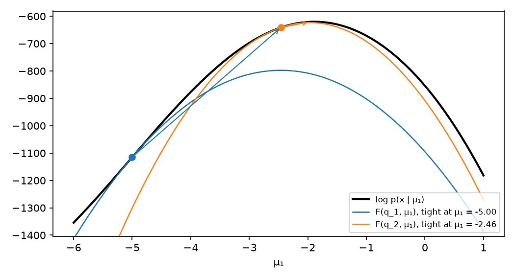
• Run. Starting from \mu_1=-5, two EM steps, drawing the bound after each E-step.

• Code Snippet

  import matplotlib.pyplot as plt
  import numpy as np
  from scipy.special import logsumexp, xlogy
  from scipy.stats import norm
  
  # 1D mixture of two unit-variance Gaussians with equal weights.
  # Only the first mean mu1 is unknown; mu2 = 2 is held fixed.
  rng = np.random.default_rng(0)
  x = np.concatenate([rng.normal(-2, 1, 150), rng.normal(2, 1, 150)])
  log_pi, mu2 = np.log([0.5, 0.5]), 2.0
  
  
  def log_joint(mu1):
      """log p(x_n, z_n = k | mu1), shape (N, 2)."""
      return log_pi + norm.logpdf(x[:, None], np.array([mu1, mu2]), 1.0)
  
  
  def loglik(mu1):
      """log p(x | mu1) = sum_n log sum_k p(x_n, z_n = k | mu1)."""
      return logsumexp(log_joint(mu1), axis=1).sum()
  
  
  def e_step(mu1):
      """E-step at mu1. Returns r, shape (N, 2): r[n, k] = p(z_n = k | x_n, mu1),
      the posterior probability that point n came from component k."""
      lj = log_joint(mu1)
      return np.exp(lj - logsumexp(lj, axis=1, keepdims=True))
  
  
  def elbo(mu1, r):
      """Lower bound F(q, mu1). r is q written as a table: r[n, k] = q(z_n = k),
      shape (N, 2). Passing the output of e_step makes q the posterior."""
      return (r * log_joint(mu1)).sum() - xlogy(r, r).sum()
  
  
  def m_step(r):
      """M-step. r: the (N, 2) table from e_step. Returns the mu1 that maximizes
      F(q, mu1): the mean of x, each point weighted by r[n, 0], its probability of
      coming from component 1."""
      return (r[:, 0] * x).sum() / r[:, 0].sum()
  
  
  grid = np.linspace(-6, 1, 400)
  mu_t = -5.0
  fig, ax = plt.subplots(figsize=(7, 3.8))
  ax.plot(grid, [loglik(m) for m in grid], "k", lw=2, label="log p(x | μ₁)")
  
  for step, color in zip(range(2), ["C0", "C1"], strict=True):
      r = e_step(mu_t)  # E-step: the bound now touches log p(x | μ₁) at mu_t
      mu_next = m_step(r)  # M-step: move to the bound's maximizer
      ax.plot(grid, [elbo(m, r) for m in grid], color=color, lw=1.2,
              label=f"F(q_{step + 1}, μ₁), tight at μ₁ = {mu_t:.2f}")
      ax.plot(mu_t, loglik(mu_t), "o", color=color)
      ax.annotate("", xy=(mu_next, loglik(mu_next)), xytext=(mu_t, loglik(mu_t)),
                  arrowprops=dict(arrowstyle="->", color=color))
      mu_t = mu_next
  
  ax.set_ylim(loglik(-6) - 50, loglik(-2) + 40)
  ax.set_xlabel("μ₁")
  ax.legend(loc="lower right", fontsize=8)
  fig.tight_layout()
  fig.savefig("em_lower_bound.png", dpi=150)

• Result

  

  • Black: the log-likelihood. Each colored curve is the bound \mathcal{F}(q_{t+1},\mu_1) from the E-step at the current estimate \mu_1^{(t)}. It touches the black curve at the current estimate, and the M-step moves to its maximum.
  • Two steps already bring the estimate close to the peak of the black curve, the maximum-likelihood estimate.

EM for Gaussian Mixtures

With the general algorithm in hand, we return to the Gaussian mixture from Why EM?. Both of its steps have closed forms, which makes it the standard first example of EM.

Deriving the Updates

The model. A Gaussian mixture model (GMM) with K components has the density

p(x_n\mid\theta)=\sum_{k=1}^{K}\pi_k\,\mathcal{N}(x_n\mid\mu_k,\Sigma_k),\qquad \theta=\{\pi_k,\mu_k,\Sigma_k\}_{k=1}^{K}

with mixing weights \pi_k\ge0 and \sum_k\pi_k=1. As a latent variable model, each point first picks a component and then draws from it:

p(z_n=k\mid\theta)=\pi_k,\qquad x_n\mid z_n=k\ \sim\ \mathcal{N}(\mu_k,\Sigma_k)

Summing out z_n gives back the density above.

E-step: responsibilities. The posterior of each label is

r_{nk}=p(z_n=k\mid x_n,\theta_t)=\dfrac{\pi_k\,\mathcal{N}(x_n\mid\mu_k,\Sigma_k)}{\sum_{j=1}^{K}\pi_j\,\mathcal{N}(x_n\mid\mu_j,\Sigma_j)}

evaluated at the current parameters \theta_t.

• r_{nk} is called the responsibility of component k for point n.

• Each row of r sums to one, so it is a soft label.

With these, the expected complete-data log-likelihood is

Q(\theta,\theta_t)=\sum_{n=1}^{N}\sum_{k=1}^{K}r_{nk}\left[\log\pi_k+\log\mathcal{N}(x_n\mid\mu_k,\Sigma_k)\right]

M-step: weighted maximum likelihood. Q is the labeled log-likelihood with point n counted r_{nk} times in component k. With the effective count N_k=\sum_n r_{nk}, its maximizer is [2]:

\pi_k=\dfrac{N_k}{N},\qquad \mu_k=\dfrac{1}{N_k}\sum_{n=1}^{N}r_{nk}\,x_n,\\ \Sigma_k=\dfrac{1}{N_k}\sum_{n=1}^{N}r_{nk}\,(x_n-\mu_k)(x_n-\mu_k)^\top

These are the weight, mean and covariance of each cluster, computed with soft counts. The mean update is the fixed-point equation from Why Direct Maximization is Hard, now with the weights frozen at \theta_t.

Derivation

Q splits into a term in \pi and one term per component in (\mu_k,\Sigma_k), so each part is maximized separately.

• Weights.
  • Maximize \sum_k N_k\log\pi_k subject to \sum_k\pi_k=1.
  • With a Lagrange multiplier \lambda, setting the derivative of \sum_k N_k\log\pi_k+\lambda(1-\sum_k\pi_k) to zero gives \pi_k=N_k/\lambda.
  • Summing over k gives \lambda=N.

• Means.
  • The gradient of \sum_n r_{nk}\log\mathcal{N}(x_n\mid\mu_k,\Sigma_k) with respect to \mu_k is \Sigma_k^{-1}\sum_n r_{nk}(x_n-\mu_k).
  • Setting it to zero gives the weighted mean.

• Covariances.
  • Write \Lambda_k=\Sigma_k^{-1}. The terms of Q in \Lambda_k are:

    \dfrac{1}{2}\sum_n r_{nk}\left[\log\det\Lambda_k-(x_n-\mu_k)^\top\Lambda_k(x_n-\mu_k)\right]

  • With \partial\log\det\Lambda/\partial\Lambda=\Lambda^{-1} and \partial\,(v^\top\Lambda v)/\partial\Lambda=vv^\top, the gradient is:

    \dfrac{1}{2}\sum_n r_{nk}\left[\Sigma_k-(x_n-\mu_k)(x_n-\mu_k)^\top\right]

  • Setting it to zero gives the weighted covariance.

Relation to k-Means

• Fix every covariance to \Sigma_k=\varepsilon I and let \varepsilon\to0. The responsibility of the nearest mean tends to one and every other to zero, so the E-step becomes the hard assignment of k-means, and the mean update becomes the k-means centroid update [2].

• EM for a GMM is a soft version of k-means that also learns the shape and the weight of each cluster.

Fitting a Mixture in Python

The following code fits a three-component GMM by EM:

• Data. The 600 points of Why EM?, drawn from a known three-component mixture.

• Start. Means at three random data points, every covariance at the covariance of all data, and uniform weights.

• Stop. When the log-likelihood gains less than 10^{-8} in one step.

• Stability. The E-step works in log space with logsumexp , which avoids underflow when a point is far from every component.

• Code Snippet

  import matplotlib.pyplot as plt
  import numpy as np
  from scipy.special import logsumexp
  from scipy.stats import multivariate_normal
  
  # Data: 600 points from a 3-component Gaussian mixture in 2D
  rng = np.random.default_rng(0)
  true_pi = np.array([0.5, 0.3, 0.2])
  true_mu = np.array([[0.0, 0.0], [4.0, 4.0], [-3.0, 4.0]])
  true_Sigma = np.array([[[1.5, 0.6], [0.6, 1.0]],
                         [[1.0, -0.4], [-0.4, 1.2]],
                         [[0.6, 0.0], [0.0, 0.6]]])
  z = rng.choice(3, size=600, p=true_pi)
  X = np.array([rng.multivariate_normal(true_mu[k], true_Sigma[k]) for k in z])
  
  
  def e_step(X, pi, mu, Sigma):
      """E-step. X: data, shape (N, D). pi, mu, Sigma: current weights (K,), means (K, D)
      and covariances (K, D, D).
      Returns the responsibilities r[n, k] = p(z_n = k | x_n, θ),
      shape (N, K), and log p(X | θ)."""
      log_p = np.stack([np.log(pi[k]) + multivariate_normal.logpdf(X, mu[k], Sigma[k])
                        for k in range(len(pi))], axis=1)  # log p(x_n, z_n = k | θ)
      log_px = logsumexp(log_p, axis=1)  # log p(x_n | θ)
      return np.exp(log_p - log_px[:, None]), log_px.sum()
  
  
  def m_step(X, r):
      """M-step. X: data (N, D). r: responsibilities (N, K) from e_step.
      Returns the weighted MLE of (π, μ, Σ), each point counted r[n, k] times in component k."""
      Nk = r.sum(axis=0)  # effective number of points per component
      pi = Nk / len(X)
      mu = (r.T @ X) / Nk[:, None]
      Sigma = np.array([((r[:, k, None] * (X - mu[k])).T @ (X - mu[k])) / Nk[k]
                        for k in range(len(Nk))])
      return pi, mu, Sigma
  
  
  def fit_gmm(X, K, max_iter=500, tol=1e-8, seed=0):
      """EM for a K-component GMM on data X (N, D), from a random start set by seed.
      Stops when log p(X | θ) gains less than tol, or after max_iter iterations.
      Returns (pi, mu, Sigma), the final responsibilities r (N, K), and the log-likelihood trace."""
      rng = np.random.default_rng(seed)
      pi = np.full(K, 1.0 / K)
      mu = X[rng.choice(len(X), K, replace=False)]  # K random data points as means
      Sigma = np.array([np.cov(X.T)] * K)
      lls = []
      for _ in range(max_iter):
          r, ll = e_step(X, pi, mu, Sigma)
          lls.append(ll)
          if len(lls) > 1 and lls[-1] - lls[-2] < tol:
              break
          pi, mu, Sigma = m_step(X, r)
      return (pi, mu, Sigma), r, np.array(lls)
  
  
  if __name__ == "__main__":
      (pi, mu, Sigma), r, lls = fit_gmm(X, K=3)
      fig, axes = plt.subplots(1, 2, figsize=(11, 4))
      axes[0].scatter(*X.T, c=r @ np.array([[0.12, 0.47, 0.71], [1.0, 0.5, 0.05],
                                            [0.17, 0.63, 0.17]]), s=8)
      t = np.linspace(0, 2 * np.pi, 100)
      for k in range(3):  # 2-std ellipse of each fitted component
          vals, vecs = np.linalg.eigh(Sigma[k])
          ellipse = mu[k][:, None] + 2 * vecs @ (np.sqrt(vals)[:, None] * [np.cos(t), np.sin(t)])
          axes[0].plot(*ellipse, "k", lw=1)
      
      axes[0].set_title("points colored by responsibilities")
      axes[1].plot(lls, "C0.-")
      axes[1].set_xlabel("iteration")
      axes[1].set_ylabel("log p(X | θ)")
      axes[1].set_title("log-likelihood per EM iteration")
      fig.tight_layout()
      fig.savefig("em_gmm.png", dpi=150)

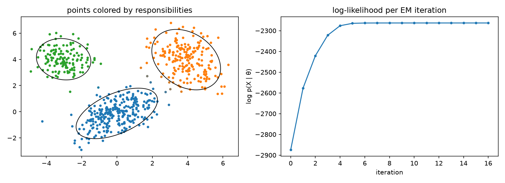
• Result

  

  • Left: the fitted 2-std ellipses. Each point is colored by mixing the three component colors with its responsibilities, so points between clusters take a blended color.
  • Right: the log-likelihood rises at every iteration, as the chain in Monotone Improvement guarantees.

Pitfalls in Practice

Monotone improvement is a strong guarantee, but it does not say which maximum EM reaches, or how fast it gets there. This section covers three common problems in practice.

Local Maxima

• Under regularity conditions, the limit points of EM are stationary points of \ell [4].

• The likelihood of a mixture usually has many such points, so the result depends on where EM starts.

The common remedies:

• Restarts. Run EM from several initializations and keep the run with the highest final log-likelihood.

• Better starts. Initialize the means with k-means, or spread the initial means apart.

Python Implementation and Result

The following code reuses fit_gmm from the previous snippet, saved as em_gmm.py :

• Data. Five well-separated clusters in 2D, 100 points each.

• Fit. A five-component GMM from 20 random starts.

• Code Snippet

  import matplotlib.pyplot as plt
  import numpy as np
  
  from em_gmm import fit_gmm  # the e_step, m_step and fit_gmm defined above
  
  # Five well-separated clusters in 2D, fitted with K = 5 from 20 random starts
  rng = np.random.default_rng(1)
  centers = np.array([[0, 0], [6, 0], [0, 6], [6, 6], [3, 3]])
  X = np.concatenate([rng.normal(c, 0.7, size=(100, 2)) for c in centers])
  
  runs = [fit_gmm(X, K=5, seed=s) for s in range(20)]
  finals = np.array([lls[-1] for _, _, lls in runs])
  
  
  def plot_fit(ax, run, title):
      """Points colored by their most likely component, with each component's 2-std ellipse."""
      (pi, mu, Sigma), r, _ = run
      ax.scatter(*X.T, c=r.argmax(axis=1), cmap="tab10", vmin=0, vmax=9, s=6)
      t = np.linspace(0, 2 * np.pi, 100)
      for k in range(len(pi)):
          vals, vecs = np.linalg.eigh(Sigma[k])
          ellipse = mu[k][:, None] + 2 * vecs @ (np.sqrt(vals)[:, None] * [np.cos(t), np.sin(t)])
          ax.plot(*ellipse, "k", lw=1)
      ax.set_title(title)
      ax.set_aspect("equal")
  
  
  i_best, i_worst = np.argmax(finals), np.argmin(finals)
  fig, axes = plt.subplots(1, 3, figsize=(14, 4.2))
  plot_fit(axes[0], runs[i_best], f"best start: log p = {finals[i_best]:.1f}")
  plot_fit(axes[1], runs[i_worst], f"worst start: log p = {finals[i_worst]:.1f}")
  at_best = np.isclose(finals, finals.max(), atol=0.1)
  axes[2].scatter(np.flatnonzero(at_best), finals[at_best], color="C0", label="best maximum found")
  axes[2].scatter(np.flatnonzero(~at_best), finals[~at_best], color="C3", label="worse local maximum")
  axes[2].legend(fontsize=8, loc="lower right")
  axes[2].set_xticks(range(0, 20, 2))
  axes[2].set_xlabel("random start (seed)")
  axes[2].set_ylabel("final log p(X | θ)")
  axes[2].set_title("where each of the 20 starts ends")
  fig.tight_layout()
  fig.savefig("em_restarts.png", dpi=150)

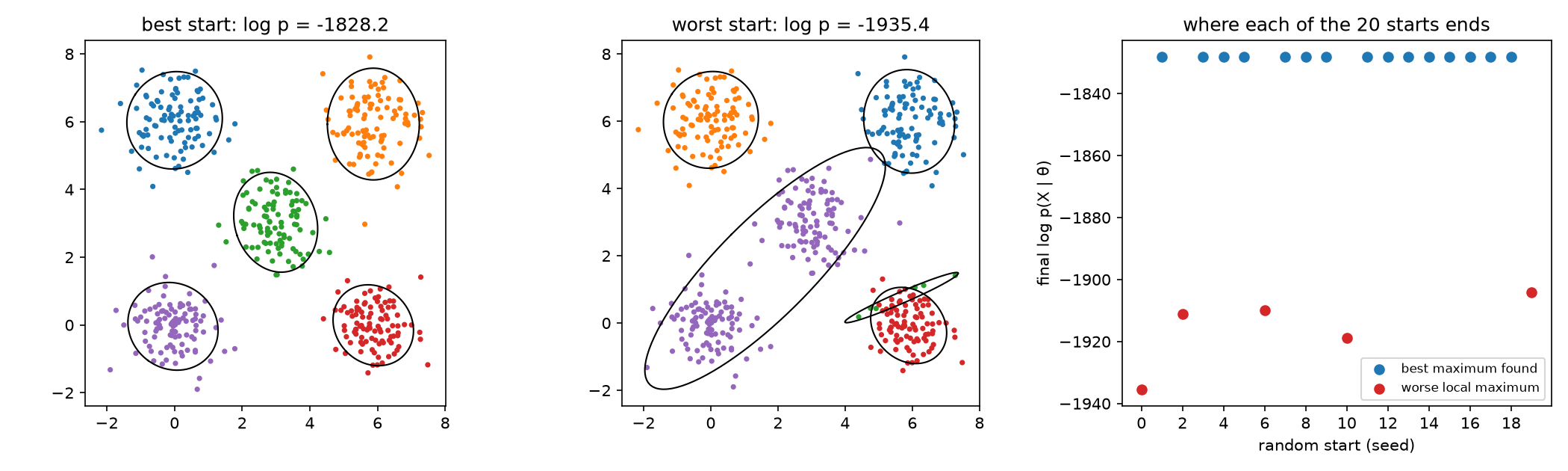
• Result

  

  • Left: the best run, one component per cluster. Most starts end here (blue dots, right).
  • Middle: the worst run. One component spans two clusters, while two components share one cluster.
  • Right: the red starts stop at such worse solutions. EM still increased the likelihood at every step: it climbed a different hill.

Degenerate Solutions

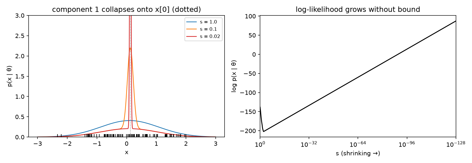
EM maximizes the likelihood because a higher likelihood is supposed to mean a better fit. For a GMM, a useless fit can make the likelihood arbitrarily large:

• Put one component's mean on a single data point and shrink its covariance toward zero.
  • That point's density grows without bound, while the other components keep every other point's density from vanishing [2].

• So the log-likelihood goes to +\infty. Ever higher scores go to a component that memorizes one point, so a global maximum does not exist.

• EM can drift there: if a component ends up with only a few points, its covariance can shrink step after step, and the run ends with a near-singular \Sigma_k and a meaningless fit.

Python Implementation and Result

The following code shrinks one component onto a single data point:

• Model. A two-component 1D mixture on 100 points. Component 1 sits on the data point x_1 with standard deviation s, and component 2 covers all the data.

• Run. Shrink s and plot the log-likelihood.

• Code Snippet

  import matplotlib.pyplot as plt
  import numpy as np
  from scipy.special import logsumexp
  from scipy.stats import norm
  
  # Two-component 1D GMM. Put component 1 exactly on the data point x[0]
  # and shrink its standard deviation s. Component 2 covers all the data.
  rng = np.random.default_rng(0)
  x = rng.normal(0, 1, 100)
  
  
  def loglik(s):
      log_p = np.stack([np.log(0.5) + norm.logpdf(x, x[0], s),
                        np.log(0.5) + norm.logpdf(x, x.mean(), x.std())], axis=1)
      return logsumexp(log_p, axis=1).sum()
  
  
  fig, axes = plt.subplots(1, 2, figsize=(11, 3.8))
  grid = np.linspace(-3, 3, 2000)
  for s, color in [(1.0, "C0"), (0.1, "C1"), (0.02, "C3")]:
      density = 0.5 * norm.pdf(grid, x[0], s) + 0.5 * norm.pdf(grid, x.mean(), x.std())
      axes[0].plot(grid, density, color=color, lw=1.2, label=f"s = {s}")
  axes[0].plot(x, np.zeros_like(x), "|", color="k", ms=10)
  axes[0].axvline(x[0], color="gray", ls=":", lw=1)
  axes[0].set_ylim(0, 3)
  axes[0].set_xlabel("x")
  axes[0].set_ylabel("p(x | θ)")
  axes[0].set_title("component 1 collapses onto x[0] (dotted)")
  axes[0].legend(fontsize=8)
  
  s_grid = np.logspace(0, -128, 400)
  axes[1].plot(s_grid, [loglik(s) for s in s_grid], "k", lw=1.5)
  axes[1].set_xscale("log")
  axes[1].set_xlim(1, 1e-128)  # reversed: s shrinks to the right
  axes[1].set_xticks([1, 1e-32, 1e-64, 1e-96, 1e-128])
  axes[1].set_xlabel("s (shrinking →)")
  axes[1].set_ylabel("log p(x | θ)")
  axes[1].set_title("log-likelihood grows without bound")
  fig.tight_layout()
  fig.savefig("em_singularity.png", dpi=150)

• Result

  

  • Left: as s shrinks, component 1 becomes a spike on x_1 (the dotted line, x[0] in the code) and stops covering the other points.
  • Right: at first the cheat costs more than it gains: the log-likelihood falls, because component 1 stops covering the other points.
  • But the spike's own term, -\log s, has no ceiling. It grows by about \log 10\approx2.3 per tenfold shrink, passes the s=1 fit near s\approx10^{-30}, and keeps growing. This is why the axis runs so far.
  • The usual fixes are a floor on the variances, a small \epsilon I added to each \Sigma_k, or a prior on \Sigma_k, which turns the problem into MAP estimation (see Relaxing the Two Steps).

Slow Convergence

Near a maximum, EM converges linearly: the error shrinks by a roughly constant factor per step. DLR show that this factor is set by the fraction of missing information, how much of the complete-data information about \theta the latent variables carry [1].

• Well-separated clusters leave little missing information. The responsibilities are close to 0 or 1, and EM converges quickly near the maximum.

• Heavily overlapping clusters leave much of it missing, and EM can crawl for many iterations.

Beyond Exact EM

Everything so far assumed that both steps can be solved exactly. This section relaxes that assumption, ending with the variational methods that connect EM to the VAE.

Relaxing the Two Steps

The E-step and the M-step need not be solved exactly. Each variant below changes one of them, and each still climbs a lower bound: \mathcal{F}(q,\theta), or \mathcal{F}(q,\theta)+\log p(\theta) for MAP-EM.

variant	E-step	M-step	guarantee
EM	exact posterior	maximize Q(\theta,\theta_t)	\ell(\theta) never decreases
MAP-EM	exact posterior	maximize Q(\theta,\theta_t)+\log p(\theta)	\log p(\theta\mid x) never decreases
generalized EM (GEM)	exact posterior	any \theta with Q(\theta,\theta_t)\ge Q(\theta_t,\theta_t)	\ell(\theta) never decreases
partial E-step (incremental, sparse)	posterior updated for only part of z	maximize \mathcal{F}(q,\theta)	\mathcal{F}(q,\theta) never decreases
variational EM	best q in a restricted family	maximize \mathcal{F}(q,\theta)	\mathcal{F}(q,\theta) never decreases

• MAP-EM adds a prior p(\theta). The same chain holds for the log posterior, since the prior term does not involve z [1].
  • A prior on the covariances is one fix for the degenerate solutions above.

• GEM is useful when the M-step has no closed form: any step that increases Q, such as a small enough gradient step, keeps the guarantee [1].

• Partial E-steps keep \mathcal{F} non-decreasing, though not \ell at every step. Neal and Hinton [3] use the bound to justify two such variants:
  • Incremental: for large datasets, to converge in fewer passes over the data.
    • The E-step updates one point at a time. After each point, the M-step refits \theta to all points, using that point's new posterior and the stored posteriors of the others.
    • So \theta is updated after every point instead of once per pass, as in SGD versus full-batch gradient descent.
  • Sparse: for latent variables with many possible values, to cut the cost of each E-step.
    • Usually only a few values have non-negligible probability. The E-step recomputes only how probability is split among those few, and keeps the rest frozen.
    • All values are recomputed now and then, since the few that matter change as \theta moves.

Variational EM and the VAE

The E-step needs the tractable posterior p(z\mid x,\theta). In many models, such as those with many interacting latent variables or with neural-network likelihoods, the posterior has no tractable form.

Variational EM restricts q to a tractable family and runs the same coordinate ascent:

• As in exact EM, we take q to split over points for i.i.d. data: q(z)=\prod_n q(z_n;\lambda_n).
  • So each point x_n gets its own member of the family, set by its own variational parameters \lambda_n, e.g. a mean and a variance for a Gaussian q.

• The E-step maximizes \mathcal{F}(q,\theta_t) over \lambda_1,\ldots,\lambda_N.
  • Each q(z_n;\lambda_n) becomes the member closest to p(z_n\mid x_n,\theta_t) in KL.

• The M-step is unchanged.

What is lost: the posterior is usually outside the family, so the KL gap stays positive. \mathcal{F} still increases at every step, but \ell(\theta) is no longer guaranteed to.

Amortized inference

• Variational EM refits every \lambda_n at every E-step, and a new point x_* needs its own optimization for \lambda_*.

• Amortized inference replaces the per-point parameters by one network q_\phi(z\mid x), the encoder, that maps any x to its approximate posterior:
  • The cost of inference is paid once, in training \phi, and a new point needs only one forward pass.
  • The bound becomes a function of two sets of network weights:

    \mathcal{F}(\phi,\theta)=\sum_n\mathbb{E}_{q_\phi(z\mid x_n)}\left[\log p(x_n,z\mid\theta)-\log q_\phi(z\mid x_n)\right]

The variational autoencoder (VAE) [5] builds on this. With a neural-network likelihood p_\theta(x\mid z), the decoder, it maximizes \mathcal{F}(\phi,\theta) jointly by stochastic gradient ascent instead of alternating E- and M-steps:

• The gradient step in \phi plays the role of the E-step.

• The gradient step in \theta plays the role of the M-step.

Reference

[1] Dempster, A. P., Laird, N. M., & Rubin, D. B. (1977). Maximum Likelihood from Incomplete Data via the EM Algorithm. Journal of the Royal Statistical Society: Series B, 39(1), 1–22.

https://doi.org/10.1111/j.2517-6161.1977.tb01600.x

[2] Bishop, C. M. (2006). Pattern Recognition and Machine Learning, ch. 9 "Mixture Models and EM". Springer.

https://www.microsoft.com/en-us/research/publication/pattern-recognition-machine-learning/

[3] Neal, R. M., & Hinton, G. E. (1998). A View of the EM Algorithm that Justifies Incremental, Sparse, and Other Variants. In Learning in Graphical Models, 355–368. Springer.

https://doi.org/10.1007/978-94-011-5014-9_12

[4] Wu, C. F. J. (1983). On the Convergence Properties of the EM Algorithm. The Annals of Statistics, 11(1).

https://doi.org/10.1214/aos/1176346060

[5] Kingma, D. P., & Welling, M. (2014). Auto-Encoding Variational Bayes. ICLR.

https://arxiv.org/abs/1312.6114