Neural Solver Towards Future of Simulation: Deep Dive
Date: 08-09-2024 | Author: Ki-Ung Song
Neural Solver Towards Future of Simulation Series
-
Neural Solver Towards Future of Simulation: Deep Dive - Current Post
-
Neural Solver Towards Future of Simulation: Exploration
-
Neural Solver Towards Future of Simulation: Intro
In previous post, we explored Neural ODEs and PINNs approaches for neural solvers.
In this post, we examine Neural Operator, a method that opens up new possibilities for efficient and accurate simulations.
Additionally, practical applications of these previously introduced neural solvers will be presented to showcase their real-world potential.
Neural Operator
Neural Operators (NOs) leverage the power of DL to model the underlying functions and mappings directly. This approach is called operator learning.
Operator Learning Intro: DeepONet
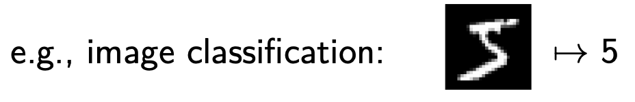
The term “operator learning” may not be clear at first glance. We will illustrate this concept with the example of DeepONet, one of the milestone achievements in operator learning.
- Good examples and illustrations from DeepONet: Learning nonlinear operators (lululxvi.github.io) will be introduced here.
Function vs. Operator
-
Function:
\R^{d_1} → \R^{d_2}
: Below is a function for
\R^{28 \times 28} \rightarrow \R^{10}
.
DeepONet: Learning nonlinear operators (lululxvi.github.io)
-
Operator:
\text{function} (∞-\dim) \mapsto \text{function} (∞-\dim)
- Derivative (local): x(t) \mapsto x'(t) .
- Integral (global): x(t) \mapsto \int K(s, t)x(s)ds .
- Dynamic system: Differential equation
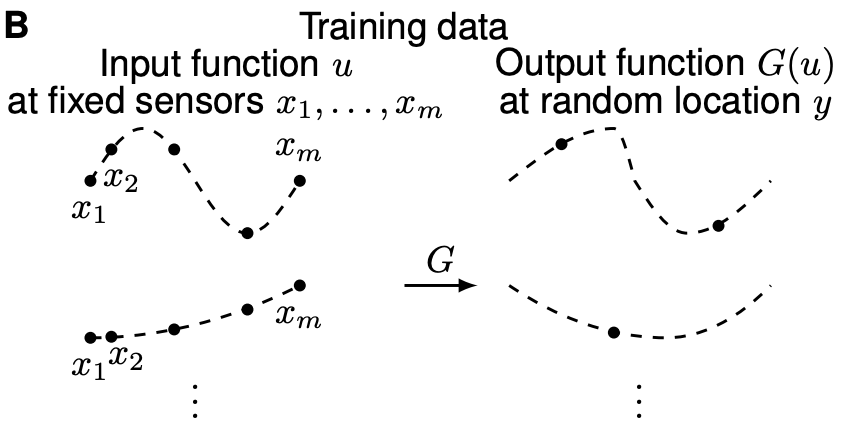
Problem Setup
The goal is to learn an operator G that maps a function u to another function G(u) . Formally:
More concretely, given a differential equation of form:
We want operator G:u \mapsto s .
-
Inputs:
u
at sensors
\{x_1, x_2, \cdots, x_m\}
and
y ∈ \R^d
.
- What exactly input x and y look like? It depends on the given DE.
-
Output:
G(u)(y) ∈ \R
.
DeepONet: Learning nonlinear operators (lululxvi.github.io)
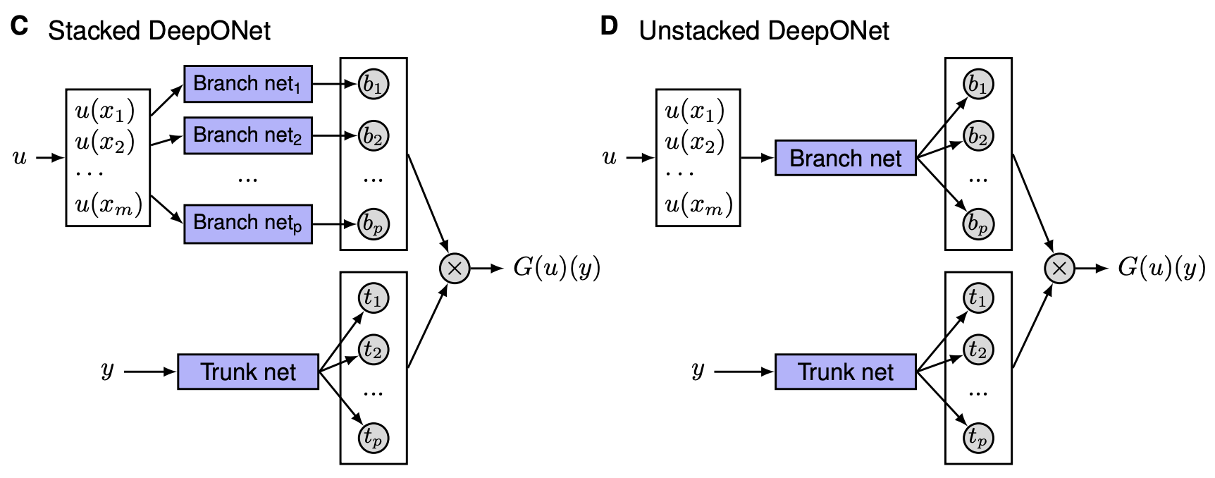
Architecture
DeepONet consists of two encoder networks:
- Branch Net : Encodes the input function into a latent representation. i.e. this encoder is used for encoding the discretized input function.
-
Trunk Net
: Encodes the coordinates or specific points where the output is evaluated. i.e. the second encoder is used for encoding the location of the output functions.
DeepONet: Learning nonlinear operators for identifying differential equations based on the universal approximation theorem of operators (arxiv.org)
The goal is to approximate the target operator G with a NN G_{\theta} :
- Prior knowledge: u and y are independent.
-
G(u)(y)
is a function of
y
conditioning on
u
.
- Branch net: b_k(u) , u -dependent coefficients.
- Trunk net: t_k(y) , basis functions of y .
Example Case: Diffusion-reaction system
Given a PDE:
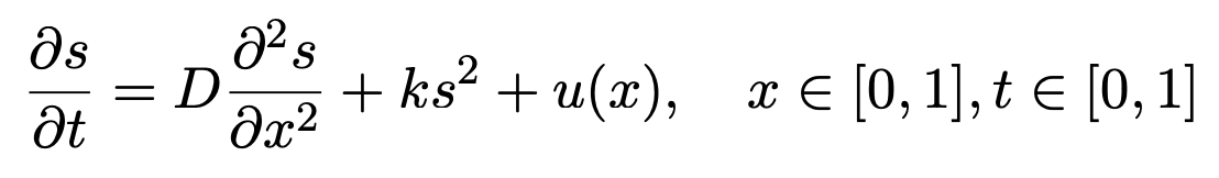
Input for branch net becomes u(x_i) and input for trunk net becomes (x_i,t_i) .
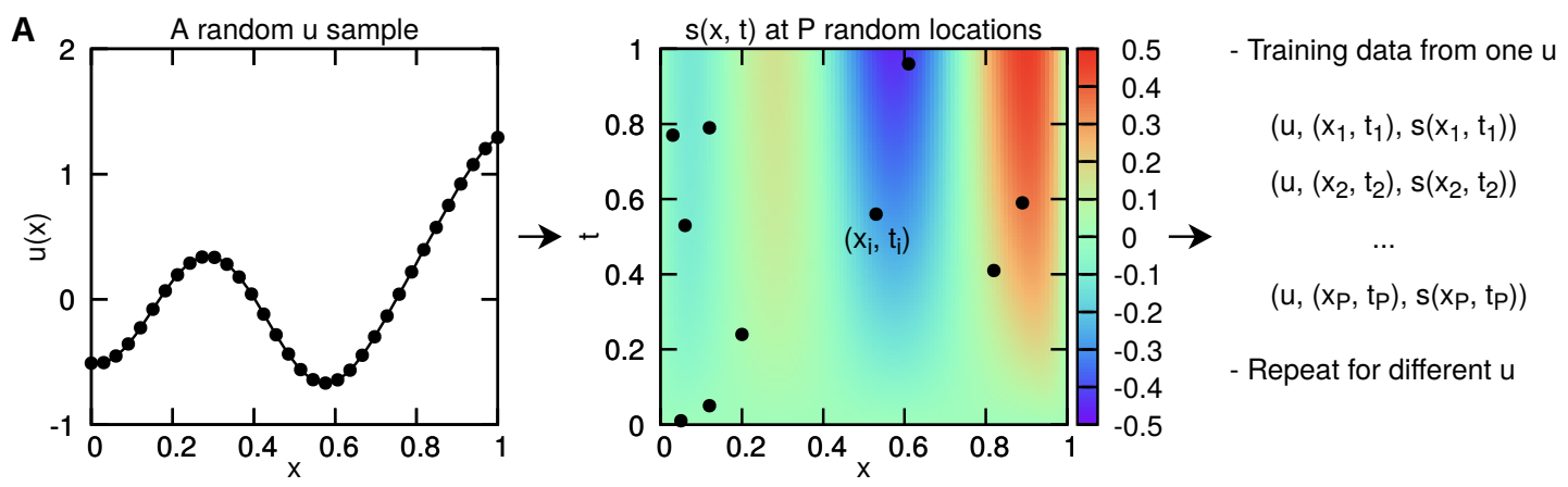
-
For a fixed function
u:\R \rightarrow \R
,
P
points are sampled for each
(x_i,t_i)
with input function estimation
u(x_i)
and solution function
s(x_t,t_i)
obtained via simulation:
\left((x_i,t_i), u(x_i), s(x_i,t_i)\right)
- Number of total dataset: \text{number of function }u \times P .
The NN output approximates as: G_\theta(u)(x_i,t_i) \approx s(x_i,t_i) .
- A naive data-driven supervised loss can be used.
- A physics-informed loss can also be used.
Discussion
-
DeepONet introduces a theorem ensuring it is a universal approximator for operator learning. This theorem underpins DeepONet's ability to accurately learn and generalize mappings between infinite-dimensional spaces.
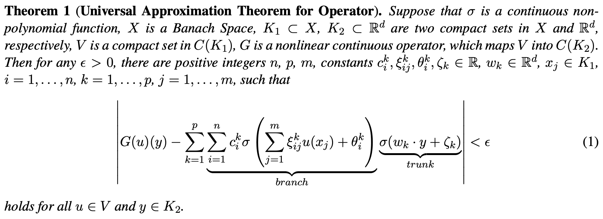
DeepONet: Learning nonlinear operators for identifying differential equations based on the universal approximation theorem of operators (arxiv.org)
-
Pros
- Accurately approximates mappings between infinite-dimensional spaces.
- Efficient for real-time simulations once trained.
-
Cons
- Requires a large amount of training data.
- Not resolution invariant; only takes input functions at a fixed discretization.
Motivation
Now, let's dive into an important milestone for neural solvers in operator learning: Neural Operators. The DeepONet from last section is also considered as a neural operator in nowadays.
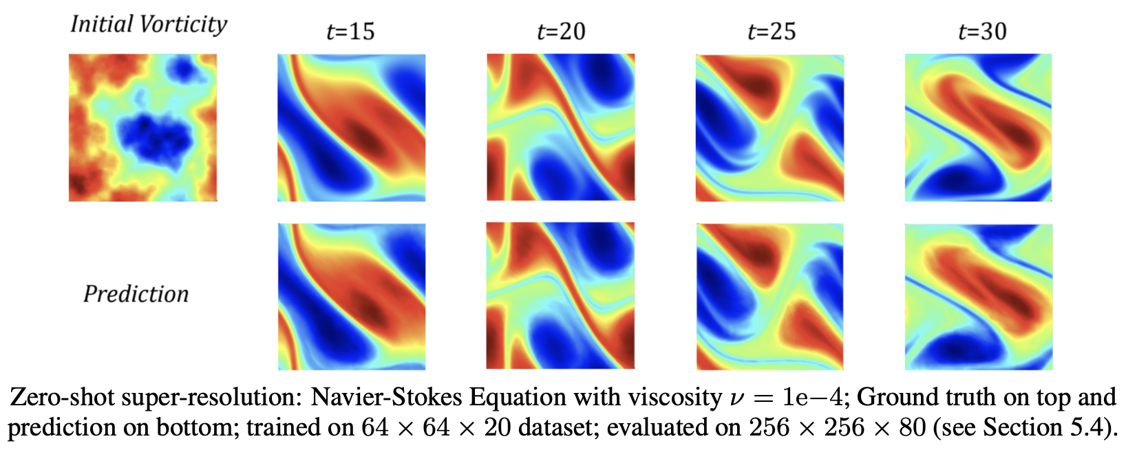
However, we'll discuss it in the context of the original Neural Operator paper: Neural Operator: Learning Maps Between Function Spaces (arxiv.org) . In this context, the following figure highlights that DeepONet lacks discretization invariance:
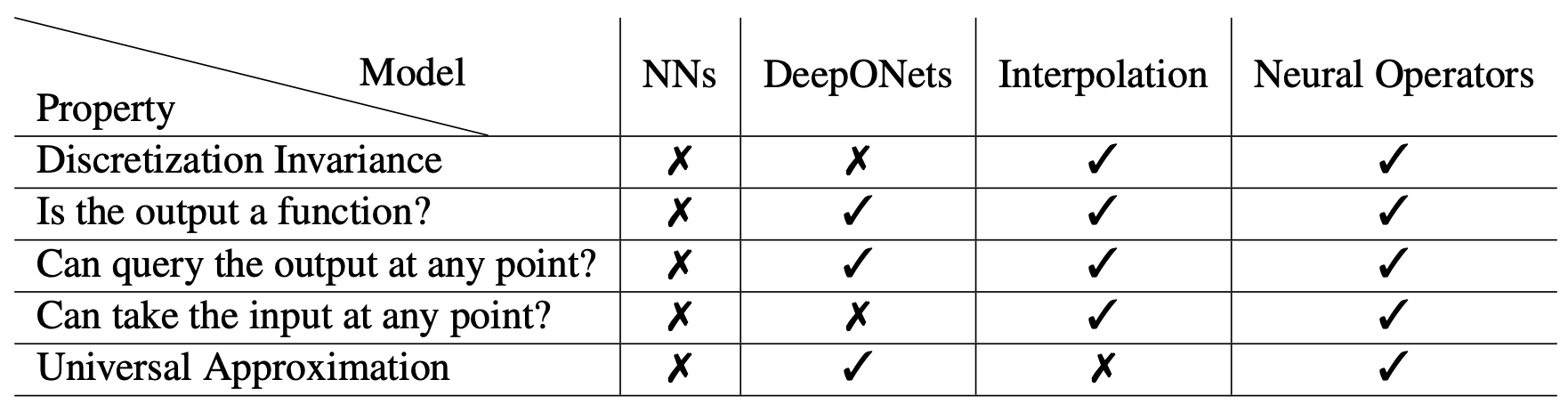
- What is discretization invariance and why it is important?
Resolution of Simulated Data
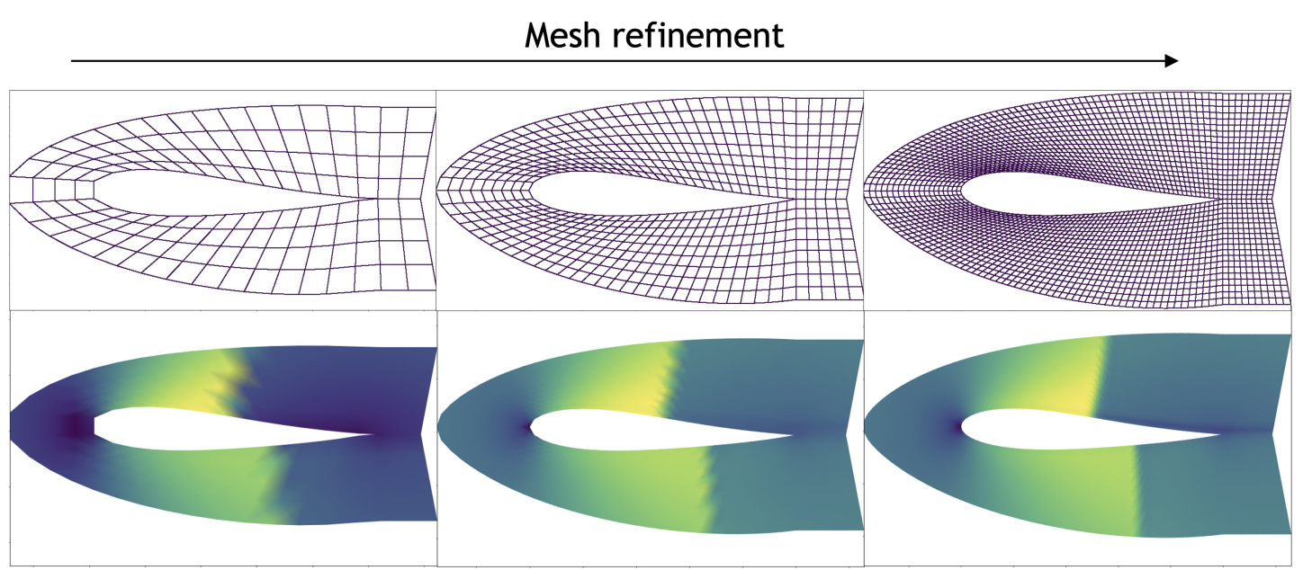
- The figure displays simulation data with increasing mesh density from left to right: sparse (low resolution), medium (medium resolution), and dense (high resolution).
- Higher resolution provides better quality simulations but requires more computational resources. Training models on low-resolution data and inferring on high-resolution data is desirable but can lead to performance degradation due to out-of-distribution issues.
- Discretization invariance allows models to handle different resolutions effectively, ensuring models trained on low-resolution data generalize well to high-resolution settings, avoiding the out-of-distribution issues that degrade performance.
Framework
Consider the generic family of PDEs:
where D ⊂ \R^d is spatial domain for the PDE with points x ∈ D in the the spatial domain.
-
e.g. Standard second order elliptic PDE
- \nabla \cdot (a(x) \nabla u(x)) = f(x), \quad x \in D \\ u(x) = 0, \quad x \in \partial D
Input function a:D\rightarrow \R^{d_a} is defined with bounded domain D and a ∈ \mathcal A .
- It includes coefficients, boundaries, and/or initial conditions.
- More concretely, initial state u_0 can be an input function.
Output function u : D' → \R^{d_u} is defined with bounded domain D'\sub \R^{d'} and u \in \mathcal U : target solution functions .
-
More concretely, solution
u_t
at some desired timestep
t
can be target solution function.
Neural Operator: Learning Maps Between Function Spaces (arxiv.org)
- We can simply assume D=D' .
Optimal operator for this PDE can be defined as \mathcal{G} = \mathcal{L}_a^{-1}f:\mathcal A \rightarrow \mathcal U : a \mapsto u . i.e. we aim to find the solution at the target timestep given initial conditions.
Theoretical Consideration
Given a linear operator \mathcal{L}_a , there exists a unique function called Green’s function G_a : D \times D \to \mathbb{R} s.t.
where \delta_x is the delta measure on \R^d centered at x .
- Note that a is denoted on G_a since it is dependent on \mathcal L_a .
Then true operator \mathcal{G} can be written as:
-
Since
\mathcal{L}_a
is linear operator with respect to variable
x
, computation order with
\int_D \cdot \, dy
can be exchanged:
f(x)= \int_D \delta_x(y) f(y) dy = \int_D \mathcal{L}_a G_a(x,y)f(y)dy \\ = \mathcal{L}_a \left(\int_D G_a(x,y)f(y)dy\right)
With fixed f , we can readily check that solution u is only dependent on input function a .
How to find such Green’s function?
If the operator \mathcal{L}_a admits a complete set of eigenfunctions (function version of eigenvector) \Psi_i(x) , i.e. \mathcal{L}_a\Psi_i=\lambda_i \Psi_i :
- Completeness means \delta(x-y)=\sum_i \Psi_i(x)^*\Psi_i(y) holds, where * denotes complex conjugation.
-
Then, the Green’s function is given by:
G_a(x,y)=\sum_i \dfrac{\Psi_i(x)^*\Psi_i(y)}{\lambda_i}
Analogous to the kernel trick in ML, G_a(x,y) can be viewed as a kernel with feature function:
This perspective of Green's function will inform the design of the neural operator layer, serving as an inductive bias, which will be introduced later.
Neural Operator Design
Main goal of neural operator is to construct NN \mathcal G_{\theta} to approximates \mathcal G .
- With discretization invariance and operator learning framework.
- Without needing knowledge of the underlying PDE.
Loss objective
Given the dataset \{a_i, u_i\}^N_{i=1} (observations), simple supervised loss is used:
Architecture
The original Neural Operator (NO) architecture has three main components:
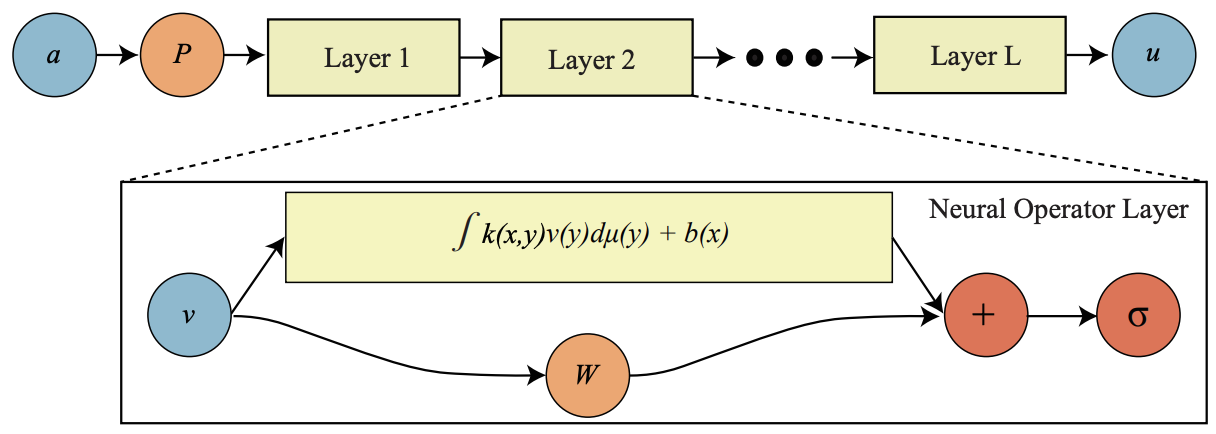
-
Lifting mapping
P
:
- P : \R^{d_a} → \R^{d_{v_0}} .
- To take advantage of NN, it sends input a_i to a high dimensional representation space.
-
Main Layer
W_i
:
- It is designed for “Iterative Kernel Integration” scheme.
- W_i: \R^{d_{v_i}} → \R^{d_{v_{i+1}}} is local linear operators.
-
Projection mapping
Q
:
- Q : \R^{d_{v_T}} → \R^{d_u} .
- Projects the high-dimensional representation back, obtaining the final solution u .
The lifting and projection mappings are straightforward. The main layer's design, based on the inductive bias of Green’s function, will be discussed in the next section.
Main Layer Design
Integral Kernel Operators
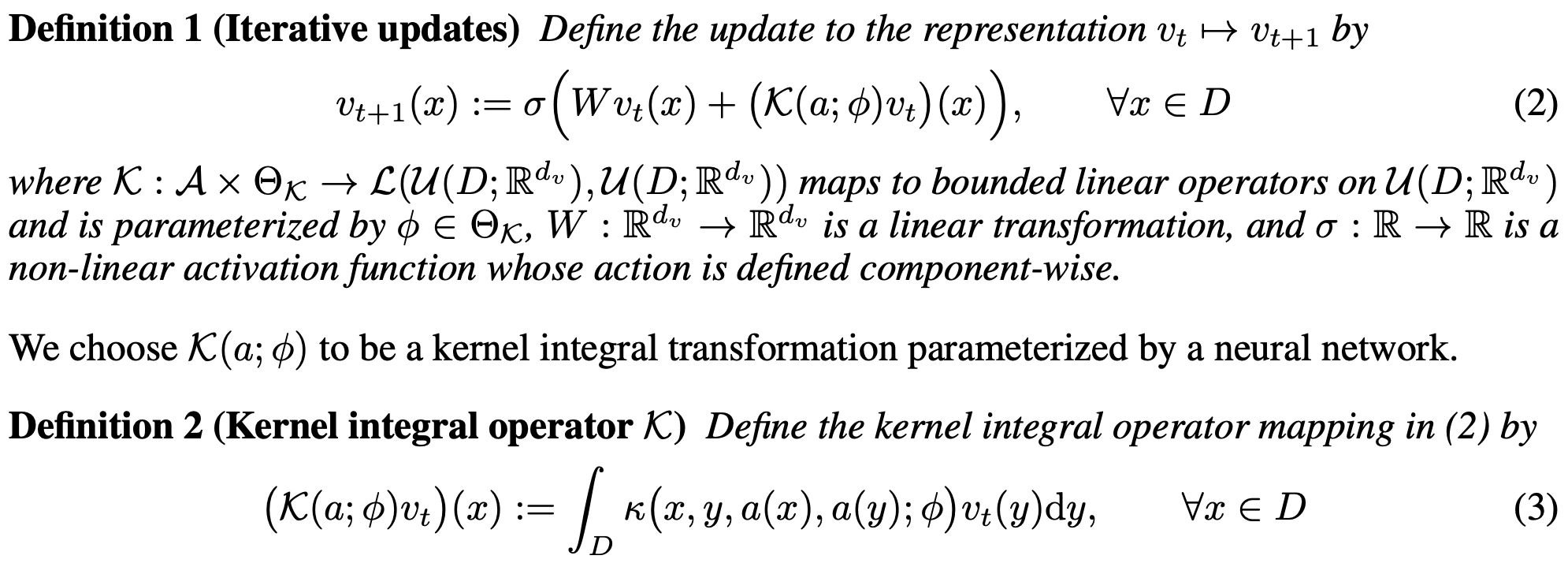
As discussed earlier, since Green's function can be viewed as a kernel, we can modify the solution u(x) = \int_D G_a(x,y)f(y) \: dy by introducing a kernel network \kappa_\phi :
Based on this, to train the NO without knowing f , we design an iterative update scheme:
where t=1,\ldots,N-1 holds.
- Here, v_t(x) and v_{t+1}(x) are input & output representation respectively.
- This iterative scheme functions as a layer of the neural operator.
The detailed design of \int \kappa_{\phi} v_t in equation (1) leads to various NO layer versions, resulting in different NO variants. This section will introduce the FNO, as proposed in the original paper.
FNO (Fourier Neural Operator)
-
Let’s follow the expression of the original paper:
Neural Operator: Learning Maps Between Function Spaces (arxiv.org) 
-
Convolution Theorem
-
Recall the definition of convolution:
f*g=\int f(x)g(y-x)dx
.
- The kernel integral operator can be seen as a convolution operator: \mathcal K(\phi)v_t \approx K(\phi) * v_t .
-
Convolution transforms to multiplication under Fourier Transform (FT):
- \mathcal{F}(f *g) = \mathcal{F}(f)\mathcal{F}(g)
- f *g = \mathcal{F}^{-1}(\mathcal{F}(f)\mathcal{F}(g))
- Using FT can bypass the often intractable integral computation of convolution.
-
Recall the definition of convolution:
f*g=\int f(x)g(y-x)dx
.
Thus, FNO designs the kernel integral operator using FT for the neural operator layer.
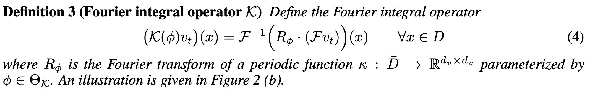
-
R_{\phi}
: Learnable transform directly parameterized in Fourier space.
- Complex-valued (k_{\max} ×d_v ×d_v) -tensor is differentiable in torch.
- FFT is also differentiable in torch: torch.fft — PyTorch 2.3 documentation .
Theoretical Consideration
Note
- For proof, lifting and projection operators Q , P are set to the identity. The authors found learning these operators beneficial in practice. Further proof to cover this is required.
- \text{NO}_n : Neural operator network with n layers.
Approximation Theorem
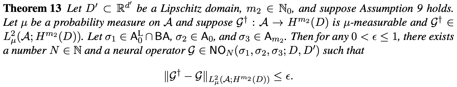
- This theorem states that a NO network with sufficient depth N can approximate any target operator G^\dagger within a specified tolerance.
- See Appendix G for detail.
Discretization Invariance
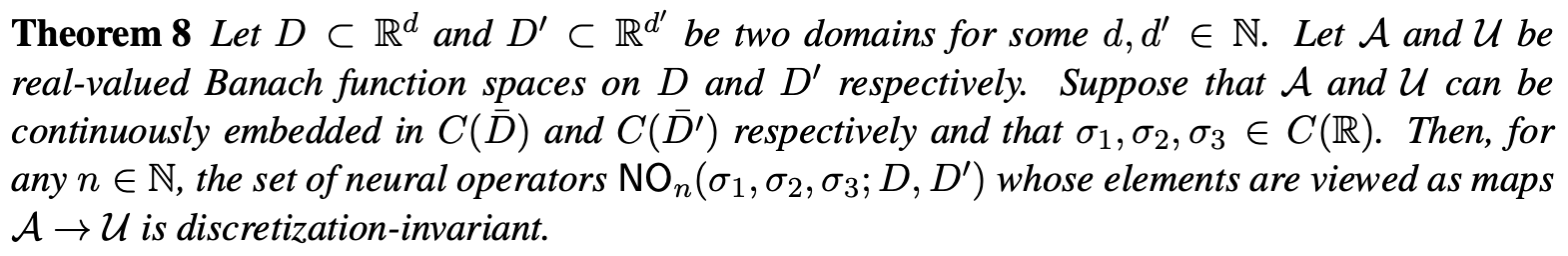
- This theorem states that NO network achieves discretization-invariance.
-
See Appendix E for detail. But let’s clarify one important thing here:
How to define discretization-invariant?
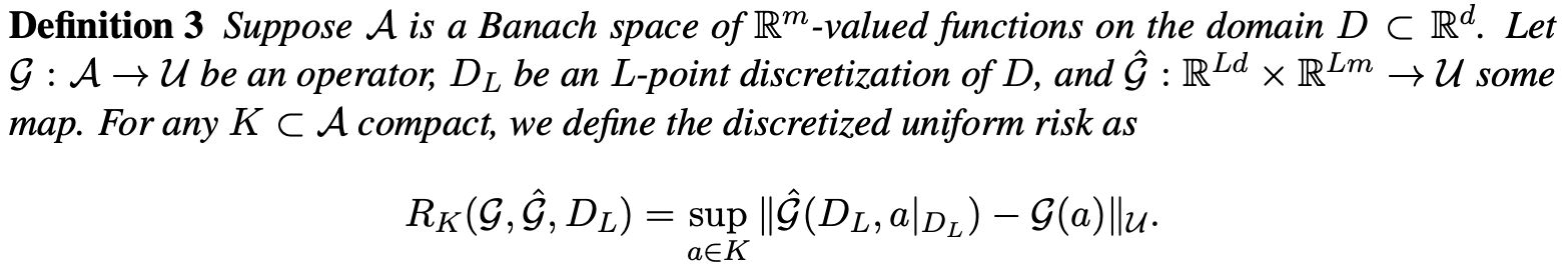
Neural Operator: Learning Maps Between Function Spaces (arxiv.org) - Even after obtaining trained \mathcal G , evaluating \mathcal G(a) is some what theoretical: Since \mathcal G is operator, input should be a function a .
-
To pass a function as input, we need to evaluate
a
on discretization
D_L
with
L
points.
- With points \{ x_1,\cdots,x_L \} , we pass function a as evaluated points \{ a(x_1),\cdots, a(x_L) \} to \mathcal G .
- We denote this discretized evaluation of a for \mathcal G as \hat{\mathcal G}(D_L, a|_{D_L}) .
- If the distance between \hat{\mathcal G}(D_L, a|_{D_L}) and \mathcal G(a) in a function space, R_K(\mathcal G, \hat{\mathcal G}, D_L) , is small for sufficiently large discretization size, then we can say \mathcal G is discretization-invariant.
-
Note that model prediction with trained NO becomes
\hat{\mathcal G}(D_L, a|_{D_L})(D_L)
naturally: e.g. mapping
\hat{\mathcal G}(D_L, a|_{D_L})(D_L) : u_0(D_L) \mapsto u_t(D_L)
.
Neural Operator: Learning Maps Between Function Spaces (arxiv.org)
Application of Neural Solvers
We will conclude this series of posts, “Neural Solver Towards the Future of Simulation,” by briefly introducing application papers on neural solvers. Figures in this section are from the respective papers.
-
FourCastNet: A Global Data-driven High-resolution Weather Model using Adaptive Fourier Neural Operators
Developed by NVIDIA, FourCastNet utilizes the Adaptive Fourier Neural Operator (AFNO) to predict weather forecasts with high resolution.
- ERA5 serves as the ground truth for comparison.
-
ClimODE: Climate and Weather Forecasting with Physics-informed Neural ODEs
| ICLR 2024 Oral
ClimODE represents 2nd-order PDEs as a system of 1st-order ODEs to apply the Neural ODE framework.


-
NN
f_\theta
is given as:
- Project Page: ClimODE (yogeshverma1998.github.io)
-
NN
f_\theta
is given as:
-
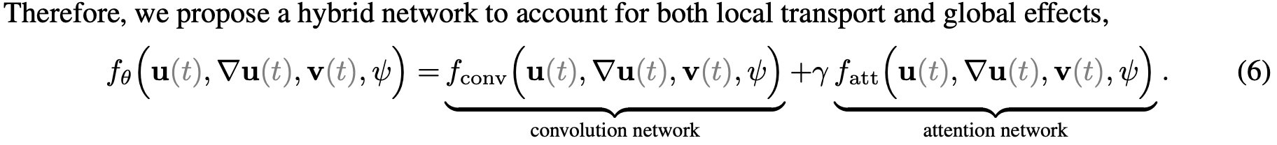
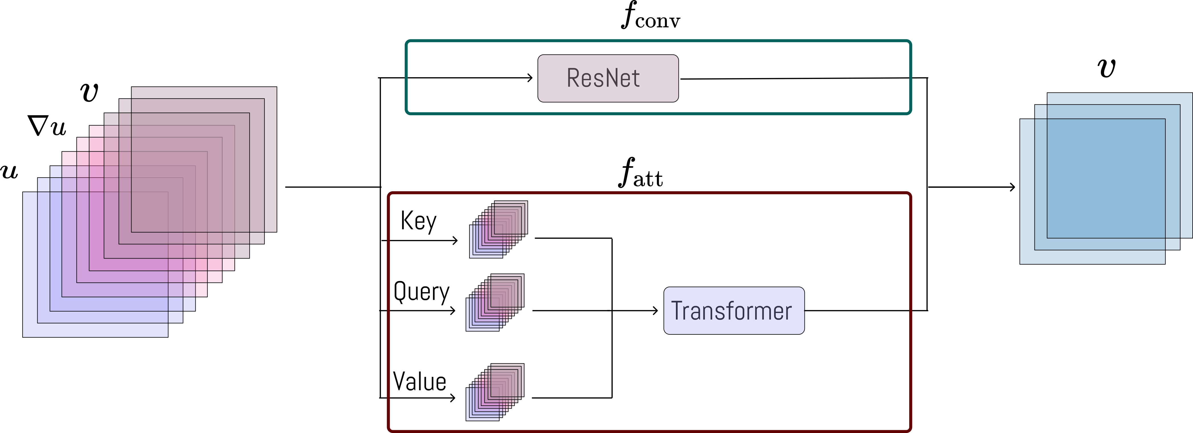
BENO: Boundary-embedded Neural Operators for Elliptic PDEs
| ICLR 2024
This neural operator architecture addresses the challenges posed by complex boundary geometries.
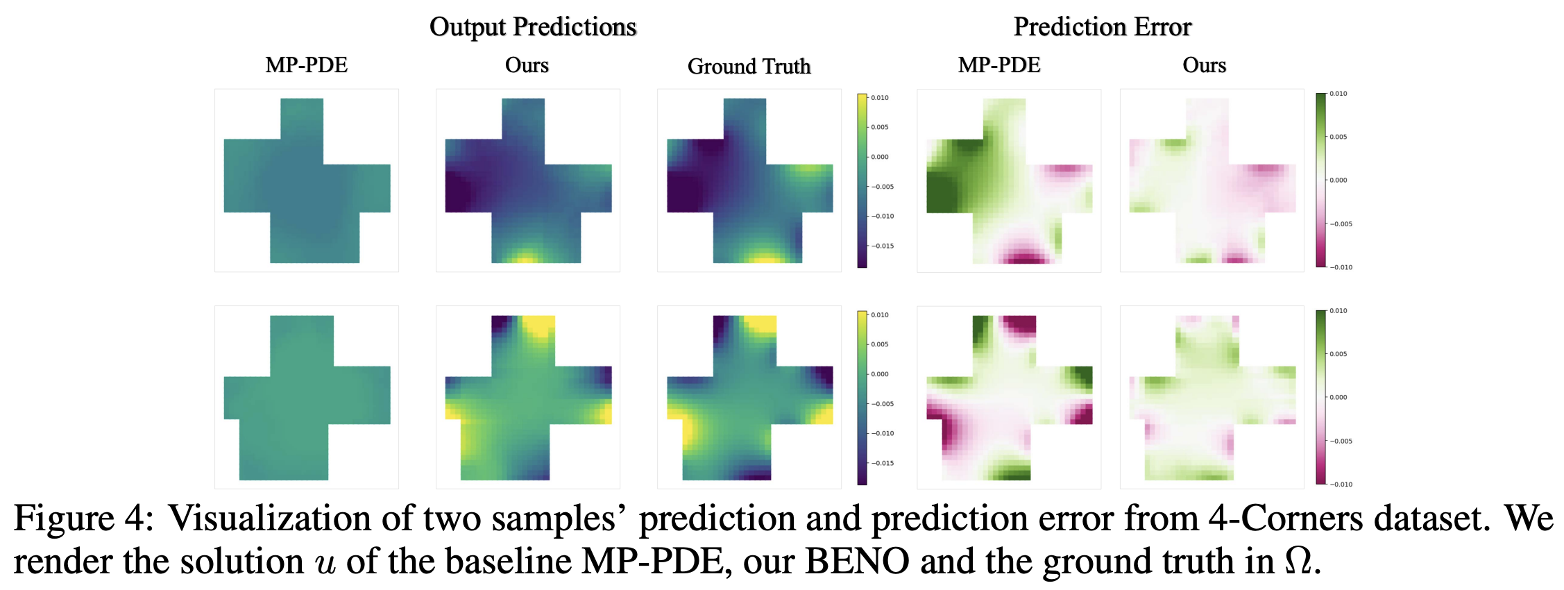
The dual-branch design builds two different types of edges on the same graph separately.
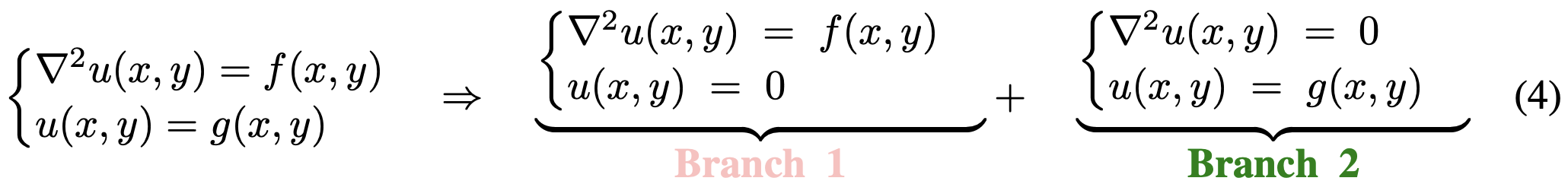
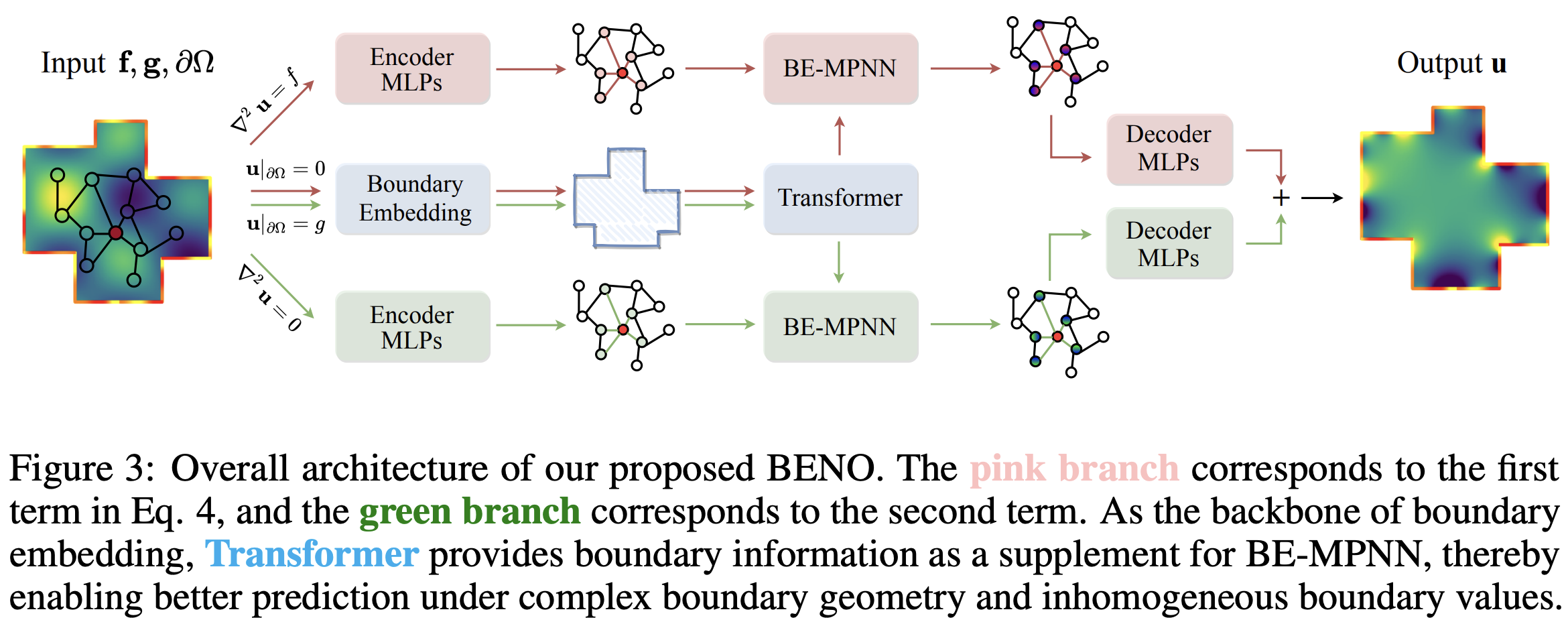
- Branch 1 considers the effects of interior nodes, governed by the Laplacian constraint.
- Branch 2 focuses solely on how to propagate the relationship between boundary values and interior nodes in the graph, dominated by the harmonic solution (zero Laplacian).