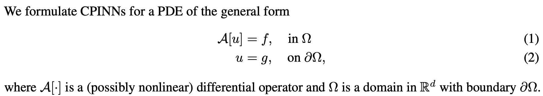
where
t ∈ \{0, \dots , T\}
,
z_t ∈ \R^D
is hidden state of
t
-th layers, and
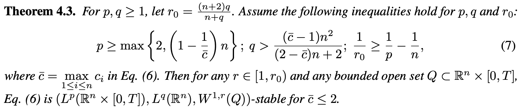
\theta_t
is
t
-th layers weight.
Recall the previously introduced Euler method:
y_{n+1} = y_n + hf(t_n, y_n)
By comparing this with the residual connection, we see a clear similarity: the residual connection can be interpreted as a single step of the Euler method with step-size
h=1
.
This allows transitioning from discrete layers to a continuous-time formulation, parameterizing the continuous dynamics between hidden states as evolving continuously over time:
Note that this can also be interpreted as a NN with infinite depth.
Forward Computation
Now we have a sophisticated formulation for NN. But how can we compute the output of this DL model explicitly? While this continuous-time approach appears elegant, it's not immediately obvious how to calculate the model's output.
Mathematical Solution:
Given initial value
z(t_0)=z(0)
, the model output
z(t_N)=z(1)
is obtained via simply integrating the both side of (1):
But you should know that integration is not a “simple” process in the real world. Integration is only mathematically meaningful, but in reality, it often turns out to be a shiny but impractical concept.
Actually, solving the differential equation is equivalent to approximating the integral in many cases. We can express the approximation of the RHS in (2) with
ODESolve()
operation. It leads to the following expression:
Assume that this kind of approximation is computed by
black-box
called “ODE solver”.
ODE solver includes basic methods like Euler method, but in practice, more sophisticated methods such as Runge-Kutta are used.
Only two observations are possible: Input
z_0
at the beginning
t_0
and output
z_1
at the end of the trajectory
t_N
since ODE solver is a black-box.
Backward Computation
But due to its black-box nature, typical
gradient computation becomes infeasible
.
It means that
{\partial z(t_N)}/\partial \theta
is not obtainable with the given
z(t_N)
, so we cannot apply chain rule to get
{\partial L}/{\partial \theta}
for weight update.
Then how can we actually train this kind of DL model? How do we apply back-propagation?
The main idea to tackle this is to approximate the gradient
{\partial L}/{\partial \theta}
for back-propagation.
Let’s find out how this becomes possible. Before that we can typical assume supervised loss with the model’s output as:
L(z(t_N)) = L \big( \text{ODESolve}(z(t_0), f_{\theta}, t_0, t_N) \big)
Recall that our goal is to approximate the gradients of
L
with respect to its parameters
\theta
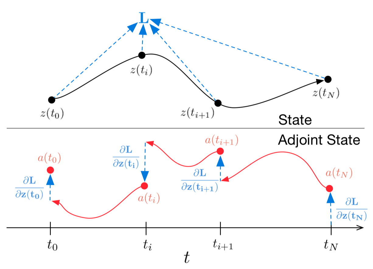
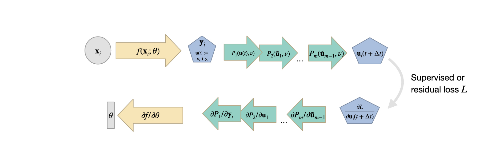
. We achieve this through step-by-step computation of various quantities, as illustrated in the figure below. You may not understand this now, but it will become clear soon.
The derived dynamics (3) is a form of ODE and from the last post, we know that the ODE can be solved reversed starting from
a(t_N)
. And it is equivalent to computing the integration in RHS of (4).
From the discussion of previous section we can expect that the integration in RHS of (4) can be approximated via ODE solver.
Step 2: Generalize again to other quantities
We can define the following quantities assuming
a_{θ}(t_N)=0
, and
\theta=\theta(t) \quad \forall t\in[0,1)
:
We can now see that solving the equation (5) reversely via computing the integration of RHS in (7) leads to the desired approximated
{\partial L}/{\partial \theta}
.
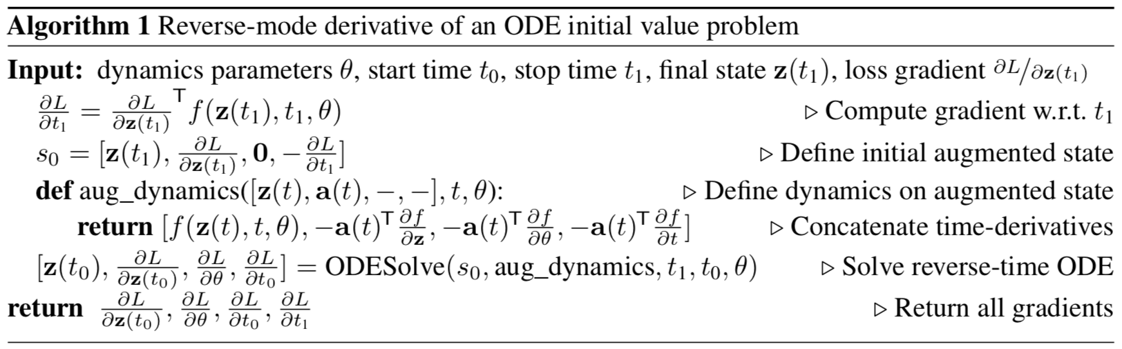
Step 3: Compute the gradient via reverse ODE solving
For reverse ODE solving, ODE solver can be used again. It should be applied to solve the following systems of the equations resulting from (1)~(8):
\begin{cases}\dot z=f_\theta(z,t),
\\
\dot a = - a \cdot \dfrac{\partial f_\theta(z,t)}{\partial z},\\
\dot a_{\theta} = - a \cdot \dfrac{\partial f_\theta(z,t)}{\partial \theta},\\
\dot a_t = - a \cdot \dfrac{\partial f_\theta(z,t)}{\partial t}.
\end{cases}
where initial values are given as:
\begin{cases}
z(t_T)= \text{Obtained at the forward pass}\\
a(t_N)=\dfrac{\partial L}{\partial z(t_N)},\\
a_{θ}(t_N)=0,\\
a_t(t_N)=a(t_N) f_\theta(t_N,z(t_N)).
\end{cases}
with
\dot{a}
is abbrev. notation for
da(t)/dt
. Same notation for others.
Why do we need to solve these many equations simultaneously?
As can be checked in the formula, the desired dynamics for
a_{\theta}
depends on
a
. Then the dynamics for
a
depends on
z
. So they need to be passed to the ODE solver simultaneously for proper computation.
Note that the dynamics
a_t(t)
can be viewed as a just dummy for gradient computation process. But this post followed the original paper’s style.
Now I believe that we can understand the above figure and the below algorithm presented in the original paper.
The above process for approximating gradients may seem complicated and limited, but thanks to many, the
ODE solver is no longer a black box. Differentiable ODE solvers are now available.
We can now apply standard backpropagation in DL as usual. So, why introduce the earlier process? I believe that understanding the original Neural ODE derivation is valuable mathematical practice.
And although differentiable ODE solvers are now available, they can’t be too heavy to apply to Neural ODEs. So, further breakthroughs are still needed.
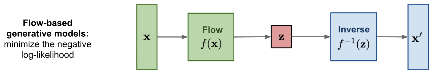
Normalizing flow is a generative model framework which involves an invertible function
f
between the data distribution space
X
and latent space
Z
.
Neural ODEs are naturally invertible due to the properties of ODEs. This allows training them in the
x\mapsto z
direction and solving them in the
z\mapsto x
direction for generation, known as
continuous normalizing flow.
This concept is related to the current flow-matching framework for diffusion models.
Solving DEs
Due to their design, Neural ODEs offer a good inductive bias for modeling and solving the dynamics of differential equations
Neural ODEs can be utilized as a key component in frameworks for Neural Solvers, enhancing their capability to handle complex differential equations efficiently.
Cases:
Optical Flow Estimation: Captures dynamic motion in video sequences.
Control Systems: Designs and analyzes stable control systems.
Climate Modeling: Predicts and models climate dynamics.
PINN (Physics-Informed Neural Network)
INR (
Implicit Neural Representation)
Implicit Neural Representation (INR) uses NNs to model continuous functions that implicitly represent data, providing a flexible and efficient way to approximate complex physical phenomena.
In other words,
INR represents signals by continuous functions parameterized by NNs
, unlike traditional discrete representations (e.g., pixel, mesh).
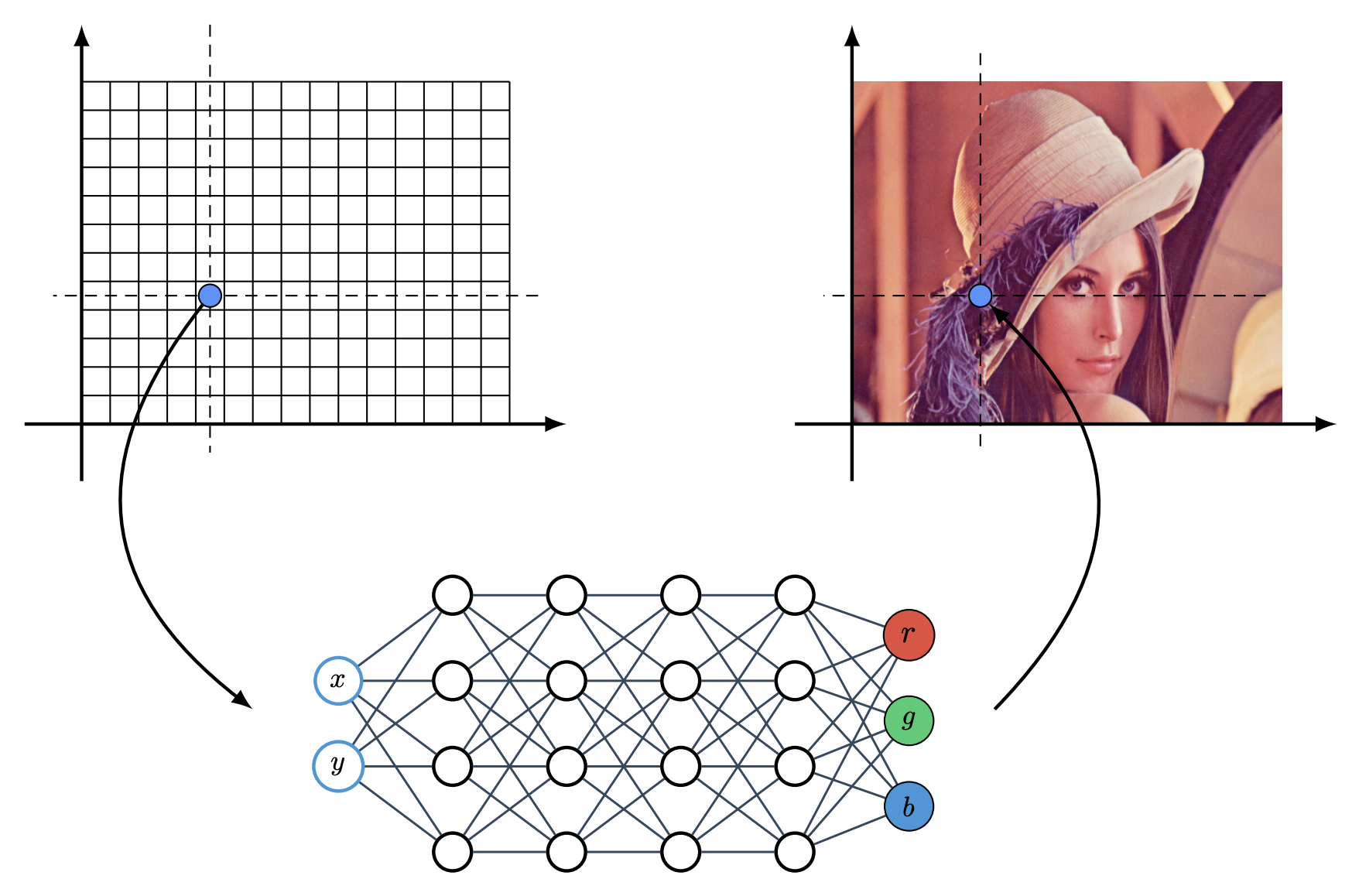
Typical RGB image data
\Omega
can be interpreted as a function: for spatial location
x\in \Omega \subset \R^2
, it corresponds to a 3-dimensional RGB value
f(x)\in\R^3
.
Given RGB image data
\Omega
, INR is a coordinate-based NN that model data as the realization of an implicit function of a spatial location
x ∈ Ω \mapsto f_θ(x)
where
f_θ:\R^2 \rightarrow \R^3
. It approximates
f_\theta \approx f
.
Consider a 1024x1024x3 image. Based on int8 representation, this image would typically require 1024×1024×3=3,145,728 bytes of memory.
And consider the above NN with 4 hidden layers of dimension 4 without bias term. Then first and last weight is
W_0\in \R^{2\times 4}
and
W_4\in\R^{4 \times 3}
respectively. And
W_i\in\R^{4\times 4}
with
i\in\{1,2,3\}
. The required memory to store the weights of this NN is 272 bytes only since there are 2x4+4x4x3+4x3=68 parameters, each needing 4 bytes (float32).
If this NN can approximate the given image properly, it significantly reduces the required memory to store the data. This is a extreme example with exaggeration, but highlights the efficiency of INR.
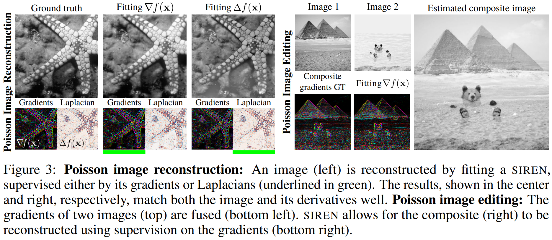
Continuous representation of INR can be obtained via physical on constraint of the data:
The above figure demonstrates how INRs can leverage physical constraints to achieve continuous and high-fidelity image reconstruction and editing.
Although the NN is fitted by physical constraints like gradient (
∇f(x)
) and Laplacian (
Δf(x)
) instead of ground truth, the reconstructions closely match the original.
This demonstrates that using a loss function based on physical constraints can efficiently approximate complex physical phenomena.
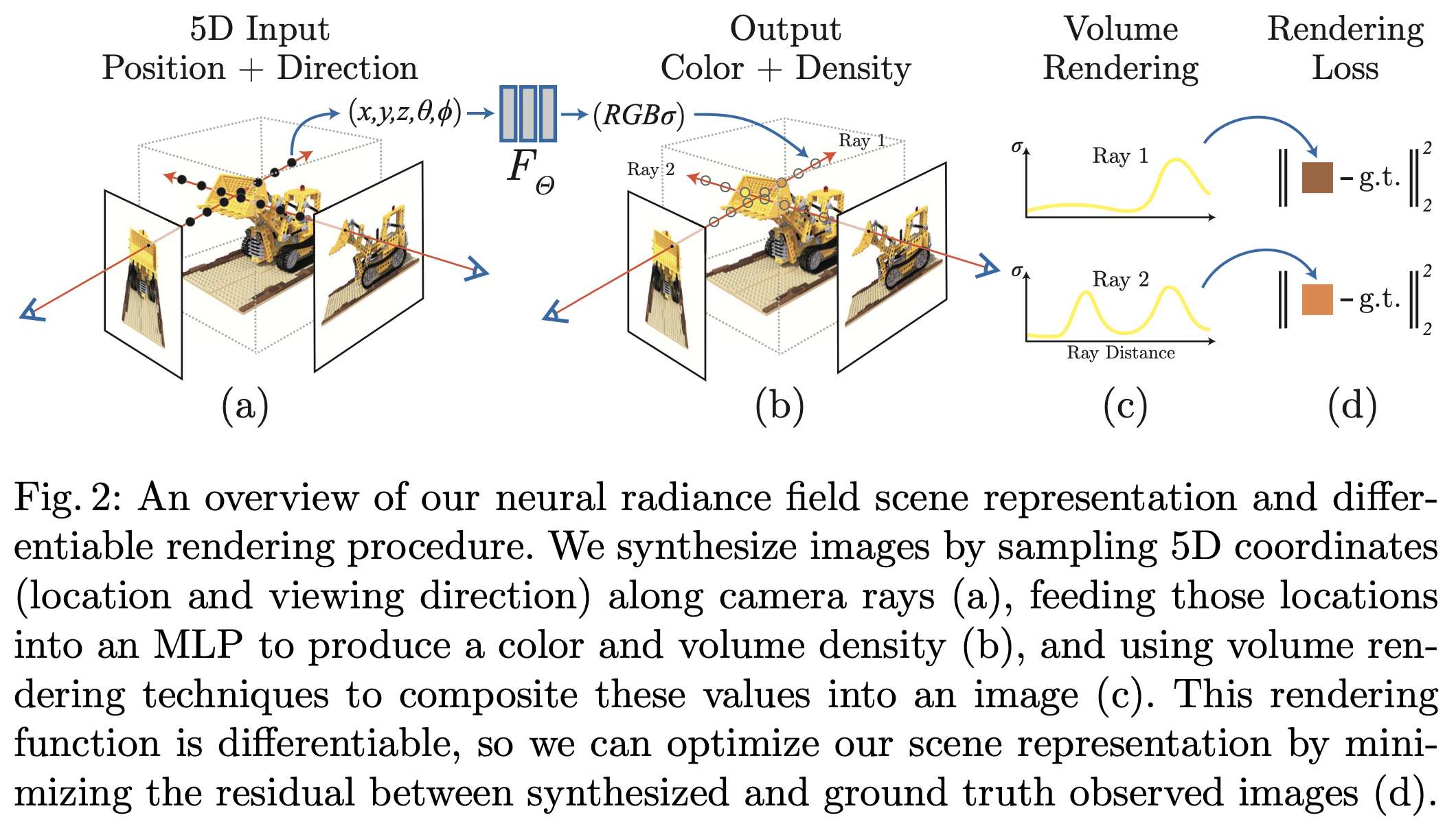
Perhaps NERF is the most famous example of an application of INRs. NERF creates continuous 5D scene representations using a Multi-Layer Perceptron (MLP) network.
The inputs are
\mathbf{x} = (x,y,z)
, representing a 3D location and
\mathbf{d}
, a 3D Cartesian unit vector. The outputs are the emitted RGB color
\mathbf{c} = (r,g,b)
and volume density
\sigma
.
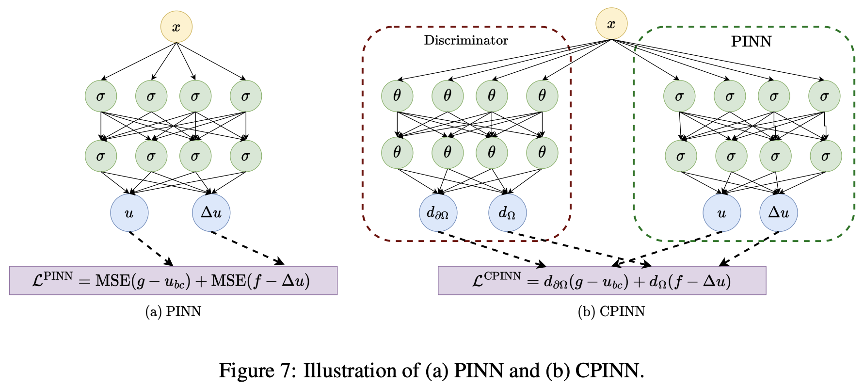
PINN
PINNs use a loss function based on physical constraints of the given data, enabling the network to learn the data itself.
This concept is fundamental to the idea of PINNs, where physical laws guide the learning process for more accurate and meaningful representations of complex phenomena.
Overview
From the previously introduced concepts, PINNs leverage the combination of physical constraints and data fitting to learn complex physical phenomena accurately.
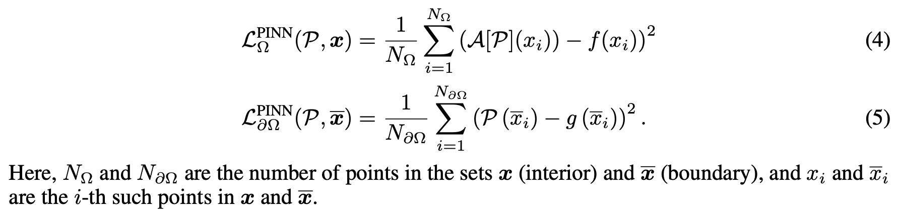
The main approach of PINNs can be expressed through the following loss function construction:
Given a PDE for
𝑢(𝑥,𝑡)
with a time evolution, we can typically express it in terms of a function
\mathcal F
of the derivatives of
𝑢
via
u_t = \mathcal F (u_{x}, u_{xx}, \cdots,u_{xx...x} ) \tag{9}
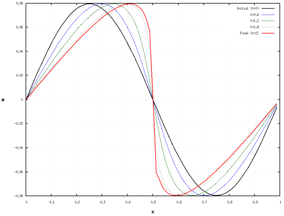
e.g. 1D Burgers Equation
\dfrac{\partial u}{\partial{t}} + u \nabla u = \nu \nabla \cdot \nabla u \tag{10}
Dataset for PINNs
The datasets used for training PINNs are typically generated by simulating the dynamics of physical system.
Dataset structure:
D=\{a_i, u_i\}^N_{i=1}
, where
a_i=(x_i,t_i)
represents the spatial and temporal variables, which are the inputs to the desired solution
u
. Specifically,
u(a_i)=u_i
.
Burgers Equation Example:
The equation (10) is known for modeling nonlinear wave propagation and shock wave formation. The data points
(a_i,u_i)
capture the evolution of the wave.
Given the dataset
D=\{a_i, u_i\}^N_{i=1}
as above, it is natural to train the NN
u_{\theta}
to approximate the true solution:
u_{\theta}(a_i)\approx u_i
.
The SL ensures that the function learned by the NN not only fits the data points but also satisfies the initial and boundary conditions of the problem.
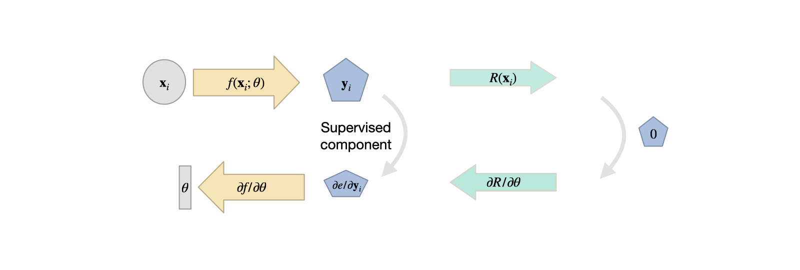
\mathcal L_{physic}
: INR Perspective
Inspired by the introduced INR, PINN represents the loss function that encapsulates the physical constraints of the problem, also known as
physic-informed loss
.
This term is crucial as it guides the neural network to learn solutions that not only fit the data but also comply with the underlying physical laws.
The required physical constraint can be obtained from PDE (9). We want the residual
R
to be zero as a constraint:
R \coloneqq u_t - \mathcal F (u_{x}, u_{xx}, \cdots,u_{xx...x} ) =0
Concrete example: For the 1D Burgers equation (10), this leads to:
R = \dfrac{\partial u}{\partial t} + u \dfrac{\partial u}{\partial x} - \nu \dfrac{\partial^2 u}{\partial x^2}
Not Generally Applicable to Any PDE:
There are numerous reported failure modes when applying PINNs to different types of PDEs.
Unstable Training:
The training process for PINNs can be unstable, making it difficult to achieve convergence and reliable results across various problem settings.
When
p
is small, such as
p=2
, which is standard for squared loss of residual as above, stable approximation cannot be obtained for some types of PDEs.
This implies that the conventional choice of
L^2
norm in the loss function may lead to instability in certain scenarios, necessitating careful design choices for PINNs.
Alternative for Physical Constraint: Differentiable Numerical Simulations
These simulations offer a promising theoretical perspective, providing a robust framework for incorporating physical constraints directly into the learning process.
Seems better in the theoretical perspective. But computationally infeasible in many cases.