Neural Solver Towards Future of Simulation: Intro
Date: 08-09-2024 | Author: Ki-Ung Song
Neural Solver Towards Future of Simulation Series
-
Neural Solver Towards Future of Simulation: Deep Dive
-
Neural Solver Towards Future of Simulation: Exploration
-
Neural Solver Towards Future of Simulation: Intro - Current Post
What is Simulation?
Everyone has likely heard the term "simulation.” But what exactly is a simulation? And how does this concept, as Elon suggests, challenge our understanding of reality and our existence? Wikipedia describes a simulation as follows.
A simulation is an imitative representation of a process or system that could exist in the real world. - Wikipedia -
So, how closely can a simulation mimic reality? With the advent of LLMs, we may think of the following scenarios when we hear “simulation”.
- From Elon's perspective, could our existence be just like the world as above, where each of us acts as objects with individual system prompts given as inputs?
- Simulation modeling like the above example is called Agent-Based Modeling (ABM) .
-
ABM provides valuable insights into economic and environmental systems:
- Individual agents, such as consumers in an economy or animals in an ecosystem, are modeled with specific behavioral rules.
- These simulations are useful for studying emergent complex outcomes from simple underlying behaviors.
ABM is an interesting topic, but today we will focus on traditional simulation methods. They can surprisingly mimic part of our reality and are widely used to solve a variety of real-world problems.
Why Simulation?
-
Paradigm Shift of Science
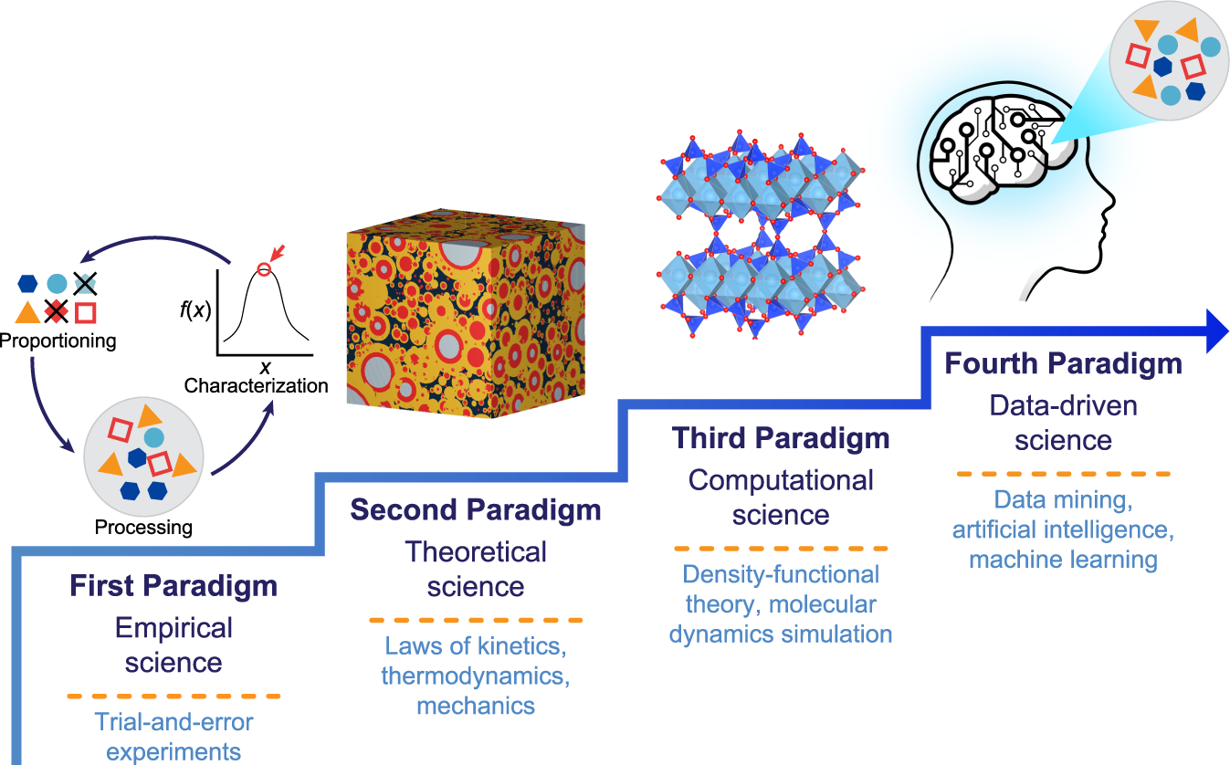
Machine learning in concrete science: applications, challenges, and best practices - Nowadays Deep Learning (DL) represents the fourth paradigm: data-driven science.
- Simulation, the third paradigm, still remains a powerful tool for predicting, analyzing, and understanding complex systems within a data-driven paradigm.
-
New paradigms do not replace existing ones; they absorb and expand upon them, complementing each other.
- e.g. Inference process of diffusion models can be viewed in a perspective of simulation. I’ll explain why in this post.
-
How DL can help?
- The current simulation framework does not effectively use existing data. Adapting these methods to leverage data-driven advantages is key to scientific development.
- DL should improve simulation quality, making it more data-efficient and faster at the same time through active use of existing data.
How Simulation Works?
The existing simulation involves creating a mathematical model that approximates real-world processes, often relying on solving various types of differential equations (DEs): ordinary (ODEs), partial (PDEs), and stochastic (SDEs).
These equations are pivotal in modeling everything from dynamic physical systems and fluid dynamics to financial models and biological processes.
Here are some detailed examples:
-
Computer Graphics: Frozen
-
In the animation film Frozen, the following PDEs are used to simulate realistic snow and ice behavior:
A Material Point Method For Snow Simulation (disneyanimation.com)
\dfrac{D\rho}{Dt}=0, \quad \rho \dfrac{D \bm{v}}{Dt} = \nabla \cdot \bm{\sigma} + \rho \bm{g}, \quad \bm{\sigma} = \dfrac{1}{J}\dfrac{\partial \Psi}{\partial \bm{F}_E} \bm{F}_E^T
-
These equations may look complicated at first glance (and indeed they are), but don't worry. You don't need to understand them. The key takeaway is that solving the PDEs results in stunning graphics that bring the scenes to life:

Disney's Frozen A Material Point Method For Snow Simulation (youtube.com)
-
For those who are interested in the PDEs, click the toggle below for details.
Details
- Snow body’s deformation can be described as a mapping from its undeformed configuration \bm{X} to its deformed configuration \bm{x} by \bm{x} = φ(\bm{X}) , which yields the deformation gradient \bm{F} = ∂φ/∂\bm{X} .
- Deformation φ(\bm{X}) changes according to conservation of mass, conservation of momentum and the elasto-plastic constitutive relation.
- ρ is density, t is time, \bm{v} is velocity, \bm{σ} is the Cauchy stress, \bm{g} is the gravity, Ψ is the elasto-plastic potential energy density, \bm{F}_E is the elastic part of the deformation gradient \bm{F} and J = \det(\bm{F}) .
-
The main idea to solve this, called material point method, is to use particles (material points) to track mass, momentum and deformation gradient.
- Specifically, each particle p holds position \bm{x}_p=(x_p, y_p, z_p) , velocity \bm{v}_p , mass m_p , and deformation gradient \bm{F}_p .
- More surprisingly, this concept is even applicable to real nature. For an in-depth exploration, check out the following: The Snow Graphics in ‘Frozen’ Can Predict the Mechanics of Real Avalanches | by Penn Engineering
-
In the animation film Frozen, the following PDEs are used to simulate realistic snow and ice behavior:
A Material Point Method For Snow Simulation (disneyanimation.com)
-
Computational Fluid Dynamics (CFD): Car Design
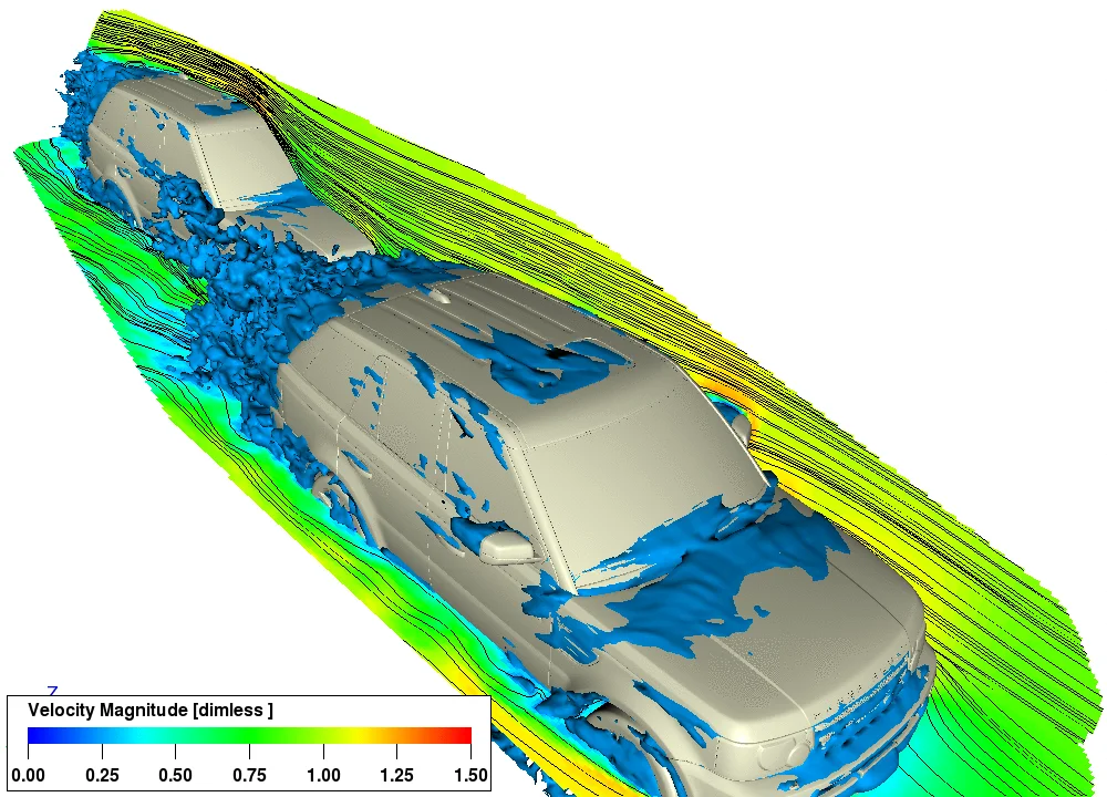
What is computational fluid dynamics? - Quora - In car design, CFD simulations use PDEs to model airflow around the vehicle, optimizing for aerodynamic efficiency and reducing drag. This enhances performance, fuel efficiency, and stability.
-
Molecular Dynamics (MD): Drug Discovery
BioSimLab - Research (uark.edu) - In drug discovery, MD simulations are used to model the interactions between atoms and molecules. This helps in understanding the behavior of biological systems at the molecular level and aids in the design of new drugs.
- Although DL models like AlphaFold are revolutionizing this domain, the predicted structure itself is not sufficient. It becomes a good starting point for further simulations as introduced above.
As seen in the examples above, simulations based on equations help solve problems by mimicking real-world phenomena in various fields. The naturally following question is how to solve these differential equations.
How to Solve Differential Equations?
-
Finite Difference Method (FDM)
- FDM is a numerical technique for solving differential equations by approximating them with difference equations. This is particularly effective for solving problems over structured grids, widely used in heat transfer and fluid dynamics.
-
The basic idea behind FDM is to replace continuous derivatives with discrete approximations:
\dfrac{\partial u}{\partial x} \approx \dfrac{u(x+h) - u(x)}{h}, \quad \dfrac{\partial^2 u}{\partial x^2} \approx \dfrac{u(x+h) - 2u(x) + u(x-h)}{h^2}
-
Euler Method
- The Euler Method can be seen as a direct application of the FDM. Despite its simplicity, it and it variants can be applied to many kinds of DEs.
-
Given the following simple form of ODE
\dfrac{dy}{dt} = f(t, y(t))
where t\in[0,1] and notation as y_0=y(0) , y_n=y(t_n) , and y_N=y(1) .
The Euler method can be expressed as
y_{n+1} = y_n + hf(t_n, y_n)where h is a step-size, i.e. t_{n+1}-t_n=h=1/N .
Now we can solve this ODE starting from the initial point y_0 . By iteratively applying the Euler method, we compute the values of y at discrete points t_n until we reach y_N .
- This process involves calculating each subsequent value y_{n+1} using the current value y_n and the function f(t_n, y_n) , progressively moving from t_0 to t_N .
-
Backward Euler method
Considering the following approximation:
y_{n+1}-y_{n}=\int_{t_{n}}^{t_{n+1}}f(t,y(t)) dt \approx hf(t_{n+1}, y_{n+1})We can derive the Euler method in reverse direction:
y_{n}=y_{n+1} - hf(t_{n+1}, y_{n+1})This implies that we can solve the ODE in the reverse direction by starting from y_{N} and iteratively applying the formula to compute previous values y_{n} , moving backward from t_{N} to t_{0} .
- Solving ODEs in reverse will be important in future content. Please remember.
-
Euler–Maruyama method
Those familiar with diffusion models should recognize the following SDE:
dx = [f_t(x) - g_t^2 \nabla_x \log p_t(x)]dt + g_t dwHow to solve this kind of SDE? The Euler–Maruyama method, a variant of the Euler Method adapted for solving SDEs, provides the simple solving process:
x_{t-1} = x_t - \gamma[f_t(x_t) - g_t^2 \nabla_{x_t} \log p_t(x_t)] + \sqrt{\gamma}g_tzwhere \gamma is a step-size and z \sim \mathcal{N}(0,1) .
- Note that this is how inference in diffusion models works.
- Recent improvements in inference speed for diffusion models are akin to faster DL-based SDE solving. In this context, we can say DL already has a strong relationship with simulation theories.
-
Finite Element Method (FEM)
-
FEM is another commonly used method to solve various DEs. It divides complex systems into smaller, simpler components known as finite elements, also referred to as the mesh method.
-
Example of a mesh grid in FEM:
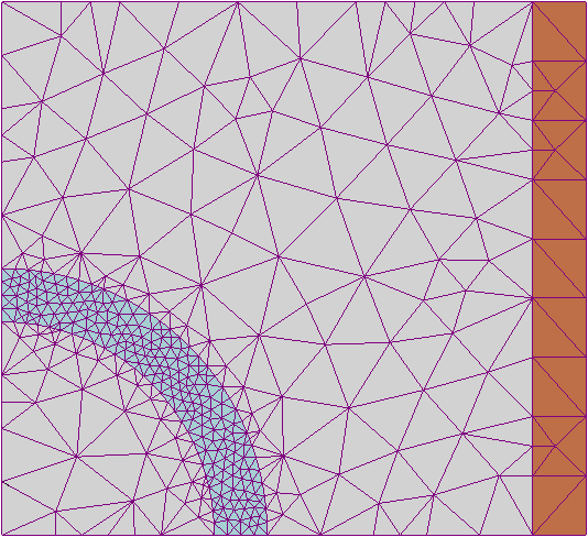
Finite element method - Wikipedia
-
Example of a mesh grid in FEM:
-
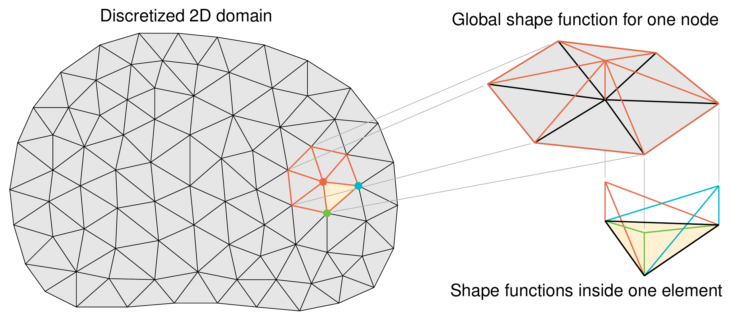
FEM aims to approximate the exact solution
u
of given PDE as a linear combination of basis (trial) functions
\{\phi_i\}_{i=1}^N
:
u \approx \tilde{u}(x) = \sum_{i=1}^N c_i \phi_i(x)
- i.e. Basis functions are used to approximate the solution over each finite element.
-
What do basis functions look like?
These functions are typically chosen for their simplicity and ability to accurately represent the solution within an element. Common basis functions include linear, quadratic, and cubic polynomials.
-
1D example: Hat function
One common type of basis function in 1D is the Hat function, which is piecewise linear. The Hat function is defined such that it is equal to 1 at a specific node and 0 at adjacent nodes, forming a 'hat' shape.
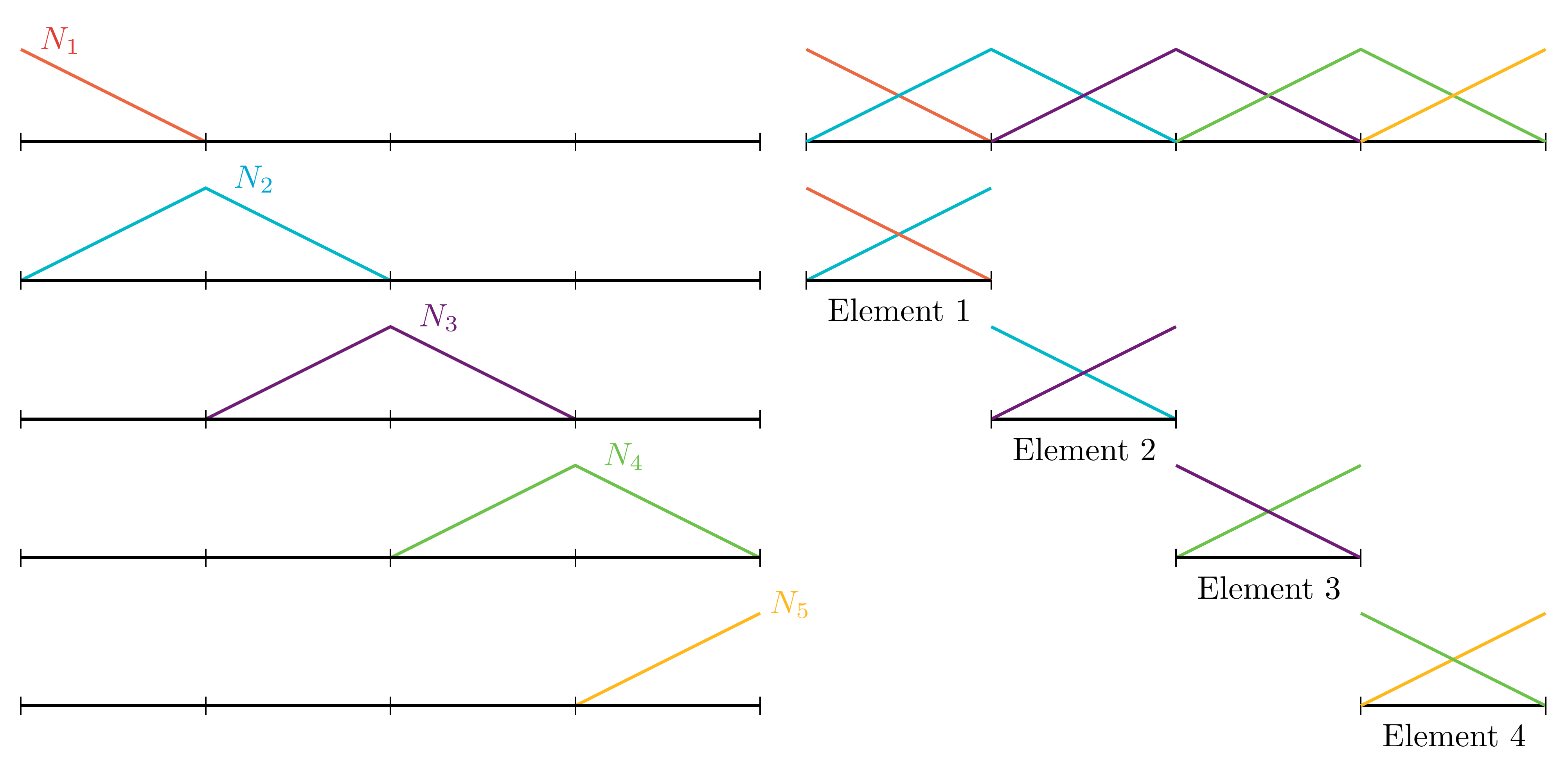
2.5. Elements and shape functions — CiTG Jupyter Book template (tudelft.nl) By finding the proper linear combination, we can visually verify that \bar{\Phi} = \sum_i N_i can approximate the given \Phi properly:
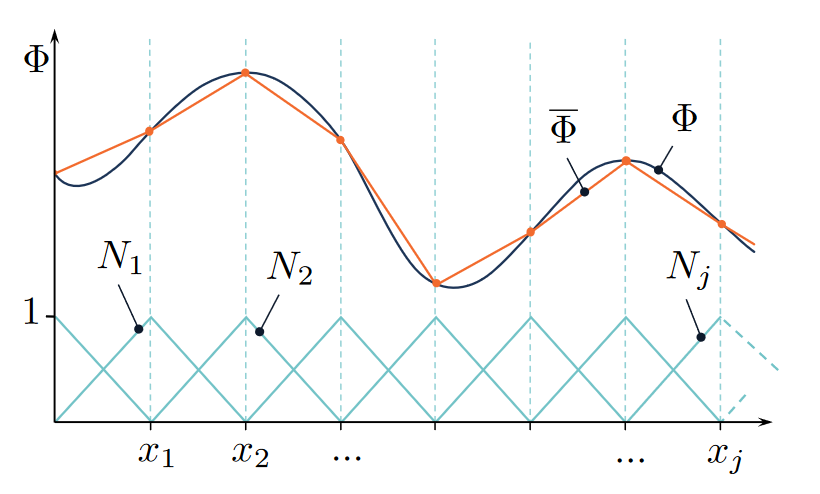
partial differential equations - Interpolation in Finite Element Method - Mathematics Stack Exchange
-
1D example: Hat function
-
The FEM method can be used with the FDM to address more complex and time-dependent PDEs.
- Combining both methods allows for efficient management of intricate geometries and dynamic systems.
- FEM offers flexible spatial discretization and FDM provides simple time integration techniques, creating a strong framework for simulating various physical phenomena.
-
FEM is another commonly used method to solve various DEs. It divides complex systems into smaller, simpler components known as finite elements, also referred to as the mesh method.
Neural Solver: DL for Solving Differential Equation
Neural solvers are DL-based frameworks designed to solve differential equations efficiently and accurately. By training and utilizing existing data from these equations, they aim to predict solutions to complex problems that are computationally intensive for traditional methods.
Trend of Accepted Papers
In recent years, the number of accepted papers on neural solvers has significantly increased. It reflects a growing interest within the scientific community. This trend highlights the potential of DL in transforming traditional problem-solving methods in mathematics and engineering.
| 2021 | 2022 | 2023 | 2024 | |
|---|---|---|---|---|
| NeurIPS | 11 | 17 | 33 | - |
| ICLR | 3 | 6 | 11 | 9 |
| ICML | 3 | 3 | 21 | 17 |
- The table is based on a survey conducted as of July 10, 2024, so it does not reflect status regarding NeurIPS 2024.
Vanilla Approach
Why don't we apply DL to the simulation data directly then? Shouldn't it work?
The content available at Supervised training for RANS flows around airfoils — Physics-based Deep Learning provides an excellent example of this and so it will be introduced here.
-
Training data:
Reynolds-Averaged Navier Stokes(RANS) around Airfoils
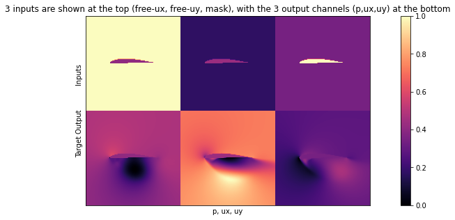
Supervised training for RANS flows around airfoils — Physics-based Deep Learning - RANS approach is a fundamental method used in computational fluid dynamics for simulation.
-
Underlying dynamics: Navier-Stokes Equation
\dfrac{\partial \mathbf{u}}{\partial{t}} + \mathbf{u} \cdot \nabla \mathbf{u} = - \dfrac{1}{\rho} \nabla p + \nu \Delta \mathbf{u} + \mathbf{g} \quad s.t. \quad \nabla \cdot \mathbf{u} = 0
where \mathbf{u} is flow velocity, p is pressure, \rho is mass density, \nu is diffusion constant for viscosity, and \mathbf{g} is body acceleration (e.g. gravity, inertia acceleration).
- The Navier-Stokes equation, known for its complexity, poses significant challenges in fluid dynamics and is one of the seven Millennium Prize Problems.
-
DL model: Simple U-net shape architecture with naive supervised loss
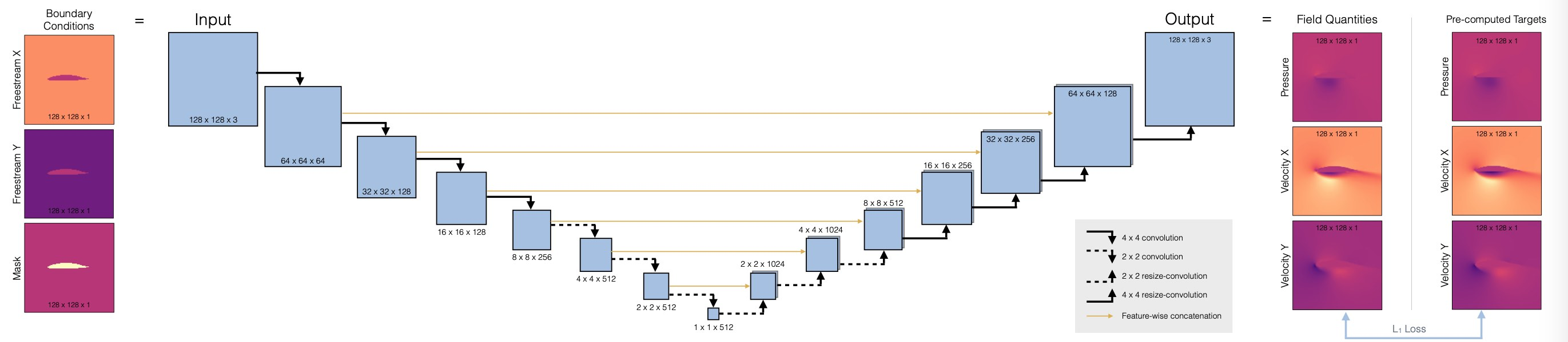
Supervised training for RANS flows around airfoils — Physics-based Deep Learning \text{arg min}_{\theta} \sum_i ( f_\theta(x_i)-y_i )^2where x_i are the boundary conditions shown on the left side of the figure, and the target y_i are the pre-computed field quantities like pressure and velocity on the right side.
-
Results: Not Optimal
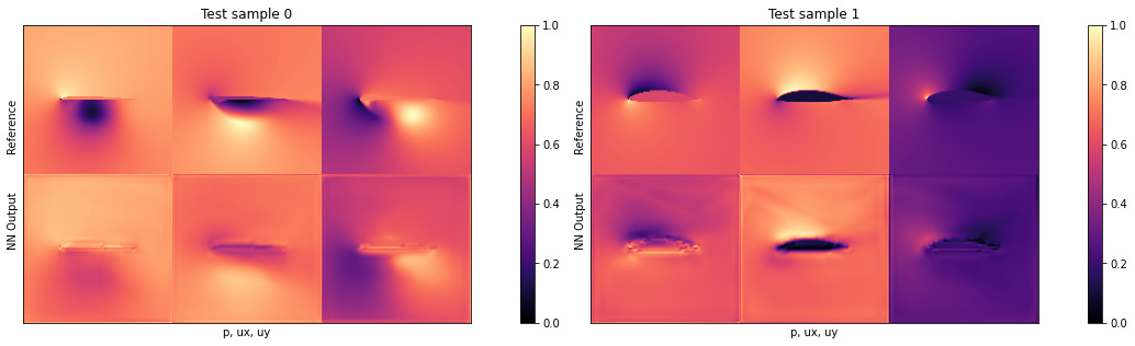
Supervised training for RANS flows around airfoils — Physics-based Deep Learning The vanilla DL approach shows limitations in capturing the complex dynamics of around airfoils, with predictions often not aligning closely with physical data, suggesting a need for more advanced models or training methods.
Next Steps in Advancing Neural Solvers
In the upcoming posts, we will explore innovative neural solver methodologies that promise greater fidelity and robustness to address the challenges shown in vanilla DL approach.
Specifically, three advanced methods will be introduced: Neural Ordinary Differential Equations (NeuralODE) , Physics-Informed Neural Networks (PINN) , and Neural Operators .
- NeuralODE represents a fusion of deep learning with differential equations, offering a continuous-time model that can dynamically adapt to the underlying physics.
- PINN incorporates physical laws into the neural network’s loss function, enhancing prediction accuracy and model generalizability.
- Neural Operators learn mappings in infinite-dimensional spaces, enabling broad applicability across different geometries and conditions.
These methods not only address traditional DL model limitations but also offer new ways to simulate complex physical systems with high precision. The upcoming post will delve into a detailed examination of each technique, their potential, and their applications.